15 Small sample tests
In the previous chapter we have seen tests for samples having size larger than 30. If the sample size \(n\) is less than 30 (\(n < 30\)), it is known as a small sample. For small samples, the sampling distributions commonly used are the \(t\), \(F\) and \(\chi^2\) (chi-square) distributions. The study of the sampling distribution of a statistic for small samples is known as small sample theory.
15.1 Tests based on Student’s t distribution (t-tests)
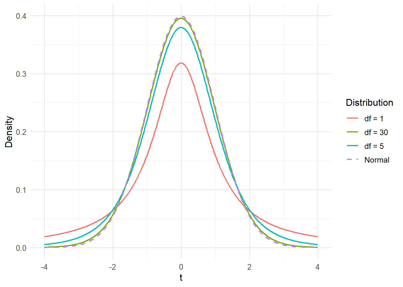
The \(t\)-distribution is a probability distribution used mainly for statistical inference when the sample size is small and the population standard deviation is unknown. It is similar to the normal distribution but has heavier tails. distribution with different degrees of freedom is shown in Figure 15.1. As the degrees of freedom increase, the \(t\) distribution converges to the standard normal distribution. \(t\)-statistic can be calculated from the sample using formulas for different situations discussed below.
Assumptions of the t-test
The parent population from which the sample is drawn is normal.
The sample is a random sample.
The population standard deviation \(\sigma\) is unknown.
15.1.1 Test for a single population mean
Consider a population with mean \(\mu\), where \(\mu\) is unknown. We take a random sample of size \(n\) (\(n < 30\)) from the population and calculate the sample mean \(\overline{x}\). We want to test whether the population mean \(\mu\) is equal to a known constant \(\mu_0\), based on the sample mean.
The null hypothesis to be tested is:
\(H_0\): \(\mu\) = \(\mu_0\)
The alternative hypothesis may be either:
\(H_1\): \(\mu\) < \(\mu_0\) (left-tailed alternative)
\(H_1\): \(\mu\) > \(\mu_0\) (right-tailed alternative)
\(H_1\): \(\mu\) \(\mathbf{\neq}\) \(\mu_0\) (two-tailed alternative)
The test statistic is:
\[t = \frac{\overline{x} - \mu_0}{\dfrac{s}{\sqrt{n}}} \tag{15.1}\]
where \(s^2 = \dfrac{\sum_{i=1}^{n}\left( x_i - \overline{x} \right)^2}{n - 1}\).
Under the null hypothesis, \(t\) follows a \(t\) distribution with \(n - 1\) degrees of freedom.
15.1.2 Decision rule for the t test
Let \(t\) be the calculated value, degrees of freedom = \(n - 1\), and \(\alpha\) be the level of significance. We reject the null hypothesis if:
\(|t| > t_{\alpha/2}\) ; for a two-tailed test
\(t > t_{\alpha}\) ; for a right-tailed test
\(t < -t_{\alpha}\) ; for a left-tailed test
Here \(t_{\alpha}\) or \(t_{\alpha/2}\) is obtained from the table of Student’s \(t\) distribution for the given degrees of freedom \(n - 1\) and level of significance \(\alpha\). If the calculated value of the test statistic is greater than the critical value from the table, we reject the null hypothesis. Otherwise, we do not have enough evidence to reject it.You can see the t-table in Table 28.1 of Appendix 4
Example 15.1 Based on field experiments, a new variety of green gram is expected to give a yield of 12 quintals per hectare. The variety was tested on 10 randomly selected farmers’ fields. The yields (quintals per hectare) were recorded as 14.3, 12.6, 13.7, 10.9, 13.7, 12, 11.4, 12, 12.6, and 13.1. Do the results confirm the expectation?
Solution
Null hypothesis, \(H_0\): \(\mu\) = 12
Alternative hypothesis, \(H_1\): \(\mu\) \(\mathbf{\neq}\) 12 (two-tailed test)
Sample size (\(n\)) = 10
Sample mean, \(\overline{x}\) = \(\dfrac{\sum_{i=1}^{n} x_i}{n} = \dfrac{14.3 + 12.6 + \ldots + 13.1}{10} = \dfrac{126.3}{10} = 12.63\)
Sample standard deviation (\(s\)) = 1.0853
\(\mu_0\) = 12
Level of significance, \(\alpha\) = 0.05
The calculation of the sample mean and sample standard deviation is shown in Table 15.1.
| Sl No. | Yield | \(\left( \mathbf{x}_{\mathbf{i}} \mathbf{-} \overline{\mathbf{x}} \right)\) | \(\left( \mathbf{x}_{\mathbf{i}} \mathbf{-} \overline{\mathbf{x}} \right)^{\mathbf{2}}\) |
|---|---|---|---|
| 1 | 14.3 | 1.67 | 2.7889 |
| 2 | 12.6 | -0.03 | 0.0009 |
| 3 | 13.7 | 1.07 | 1.1449 |
| 4 | 10.9 | -1.73 | 2.9929 |
| 5 | 13.7 | 1.07 | 1.1449 |
| 6 | 12 | -0.63 | 0.3969 |
| 7 | 11.4 | -1.23 | 1.5129 |
| 8 | 12 | -0.63 | 0.3969 |
| 9 | 12.6 | -0.03 | 0.0009 |
| 10 | 13.1 | 0.47 | 0.2209 |
From Table 15.1, the sum of squared deviations is \(\sum_{i=1}^{n}\left( x_i - \overline{x} \right)^2 = 10.601\).
\[s^2 = \frac{\sum_{i=1}^{n}\left( x_i - \overline{x} \right)^2}{n-1} = \frac{10.601}{9} = 1.1779\]
\[s = \sqrt{1.1779} = 1.0853\]
The test statistic is:
\[t = \frac{\overline{x} - \mu_0}{\dfrac{s}{\sqrt{n}}} = \frac{12.63 - 12}{\dfrac{1.0853}{\sqrt{10}}}\]
\[= \frac{0.63}{0.3432} = 1.835\]
The table value of \(t\) for 9 degrees of freedom at the 5% level of significance (two-tailed) is 2.262 (see the Table 28.1 in Appendix 4).
Since the calculated value (1.835) is less than the table value (2.262), we do not have enough evidence to reject the null hypothesis. We conclude that there is insufficient evidence to say the mean differs from 12 quintals per hectare. That is null hypothesis is not rejected and the results confirm the expectation.
Exercise 15.1 The mean weekly sales of soap bars in departmental stores were 146.3 bars per store. After an advertising campaign, the mean weekly sales in 22 stores for a typical week was 153.7, with a standard deviation of 17.2. Was the advertising campaign successful? (\(\alpha\) = 0.05)
15.2 Test for equality of two means
Let there be two normally distributed populations with means \(\mu_1\) and \(\mu_2\). Let the population standard deviations be equal and unknown. Let samples of sizes \(n_1\) and \(n_2\) be taken from these populations, with sample means \(\overline{x}_1\) and \(\overline{x}_2\) respectively. We want to test whether the two population means are significantly different, based on the sample means.
There are two cases under this situation:
Population variances are equal. (Homogeneous variances)
Population variances are unequal. (Heterogeneous variances)
Before proceeding to the t-test, an F-test is performed to test the homogeneity of population variances (see Section 15.6).
When the population variances are equal (homogeneous)
The null hypothesis to be tested is:
\(H_0\): \(\mu_1\) = \(\mu_2\)
The alternative hypothesis may be either:
\(H_1\): \(\mu_1\) < \(\mu_2\) (left-tailed alternative)
\(H_1\): \(\mu_1\) > \(\mu_2\) (right-tailed alternative)
\(H_1\): \(\mu_1\) \(\mathbf{\neq}\) \(\mu_2\) (two-tailed alternative)
We calculate the test statistic \(t\) using the following formula:
\[t = \frac{\overline{x}_1 - \overline{x}_2}{s \sqrt{\dfrac{1}{n_1} + \dfrac{1}{n_2}}} \tag{15.2}\]
where \(s^2 = \dfrac{(n_1 - 1)s_1^2 + (n_2 - 1)s_2^2}{n_1 + n_2 - 2}\) is the pooled variance, and \(\overline{x}_1\) and \(\overline{x}_2\) are the sample means from populations 1 and 2 respectively.
Under the null hypothesis, \(t\) follows a \(t\) distribution with \(n_1 + n_2 - 2\) degrees of freedom. The decision rule is the same as for the previous t-test (see Section 15.1.2).
When the population variances are unequal
The Welch t-test is an adaptation of Student’s t-test. It is used to compare the means of two groups when the variances are different.
The null hypothesis to be tested is:
\(H_0\): \(\mu_1\) = \(\mu_2\)
The alternative hypothesis may be either:
\(H_1\): \(\mu_1\) < \(\mu_2\) (left-tailed alternative)
\(H_1\): \(\mu_1\) > \(\mu_2\) (right-tailed alternative)
\(H_1\): \(\mu_1\) \(\mathbf{\neq}\) \(\mu_2\) (two-tailed alternative)
We calculate the test statistic \(t\) using the following formula:
\[t = \frac{\overline{x}_1 - \overline{x}_2}{\sqrt{\dfrac{s_1^2}{n_1} + \dfrac{s_2^2}{n_2}}} \tag{15.3}\]
where \(s_1\) and \(s_2\) are the sample standard deviations from the two populations respectively.
The degrees of freedom of the Welch t-test are calculated as follows:
\[\text{df} = \frac{\left( \dfrac{s_1^2}{n_1} + \dfrac{s_2^2}{n_2} \right)^2}{\dfrac{s_1^4}{n_1^2 (n_1 - 1)} + \dfrac{s_2^4}{n_2^2 (n_2 - 1)}} \tag{15.4}\]
Once the \(t\) value is determined, read the critical value of Student’s \(t\) distribution from the table corresponding to the significance level. The decision rule is the same as for the previous t-test (see Section 15.1.2).
Exercise 15.2 In order to compare the effectiveness of two sources of nitrogen, namely ammonium chloride and urea, on the grain yield of paddy, an experiment was conducted. The results on the grain yield of paddy (kg/plot) under the two treatments are given below. Test whether the two sources differ in effectiveness. (\(\alpha\) = 0.05)
Ammonium chloride: 13.4, 10.9, 11.2, 11.8, 14, 15.3, 14.2, 12.6, 17, 16.2, 16.5, 15.7
Urea: 12, 11.7, 10.7, 11.2, 14.8, 14.4, 13.9, 13.7, 16.9, 16, 15.6, 16
15.3 Paired t-test
The paired t-test is used to compare the means of two related samples, that is, when we have two values (a pair of values) for the same experimental unit. For example, suppose 20 cows receive a treatment for 3 months and the question is whether the treatment has an impact on milk yield. The milk yield of the 20 cows is measured before and after the treatment. This gives 20 values before treatment and 20 values after treatment. To test whether there is any significant difference between before and after, the paired t-test can be used, because the two sets of values being compared are related. We have a pair of values for each cow, one before and one after treatment.
Suppose we have two correlated random samples \(x_1, x_2, \ldots, x_n\) and \(y_1, y_2, \ldots, y_n\). We want to test whether the two population means are significantly different.
The null hypothesis to be tested is:
\(H_0\): \(\mu_1\) = \(\mu_2\)
The alternative hypothesis may be either:
\(H_1\): \(\mu_1\) < \(\mu_2\) (left-tailed alternative)
\(H_1\): \(\mu_1\) > \(\mu_2\) (right-tailed alternative)
\(H_1\): \(\mu_1\) \(\mathbf{\neq}\) \(\mu_2\) (two-tailed alternative)
We calculate the test statistic \(t\) using the following formula:
\[t = \frac{\overline{d}}{\dfrac{s}{\sqrt{n}}} \tag{15.5}\]
where \(\overline{d} = \dfrac{\sum_{i=1}^{n} d_i}{n}\), \(d_i = x_i - y_i\), and \(s^2 = \dfrac{\sum_{i=1}^{n}\left( d_i - \overline{d} \right)^2}{n - 1}\).
Under the null hypothesis, \(t\) follows a \(t\) distribution with \(n - 1\) degrees of freedom. For a two-tailed test, we compare \(|t|\) with the critical value. The decision rule is the same as for the previous t-test (see Section 15.1.2).
Example 15.2 In an experiment, plots were divided into two equal parts. One part received soil treatment A and the second part received soil treatment B. Each plot was planted with sorghum. The sorghum yield (kg/plot) was observed as shown below. Test the effectiveness of the soil treatments on sorghum yield.
| Treatment A | 49 | 53 | 51 | 52 | 47 | 50 | 52 | 53 |
| Treatment B | 52 | 55 | 52 | 53 | 50 | 54 | 54 | 53 |
Solution
Null hypothesis, \(H_0\): \(\mu_1\) = \(\mu_2\) (there is no significant difference between the effects of the two soil treatments)
Alternative hypothesis, \(H_1\): \(\mu_1\) \(\mathbf{\neq}\) \(\mu_2\) (two-tailed test; there is a significant difference between the effects of the two soil treatments)
Level of significance, \(\alpha\) = 0.05
The calculation of the differences is shown in Table 15.2.
| Sl No. | \(\mathbf{A}\) | \(\mathbf{B}\) | \(\mathbf{d}_{\mathbf{i}} \mathbf{= A - B}\) | \(\mathbf{d}_{\mathbf{i}} \mathbf{-} \overline{\mathbf{d}}\) | \(\left( \mathbf{d}_{\mathbf{i}} \mathbf{-} \overline{\mathbf{d}} \right)^{\mathbf{2}}\) |
|---|---|---|---|---|---|
| 1 | 49 | 52 | -3 | -1 | 1 |
| 2 | 53 | 55 | -2 | 0 | 0 |
| 3 | 51 | 52 | -1 | 1 | 1 |
| 4 | 52 | 53 | -1 | 1 | 1 |
| 5 | 47 | 50 | -3 | -1 | 1 |
| 6 | 50 | 54 | -4 | -2 | 4 |
| 7 | 52 | 54 | -2 | 0 | 0 |
| 8 | 53 | 53 | 0 | 2 | 4 |
From Table 15.2, \(\sum_{i=1}^{8} d_i = -16\) and \(\sum_{i=1}^{8}\left( d_i - \overline{d} \right)^2 = 12\).
\[\overline{d} = \frac{\sum_{i=1}^{8} d_i}{n} = \frac{-16}{8} = -2\]
\[s^2 = \frac{\sum_{i=1}^{8}\left( d_i - \overline{d} \right)^2}{n-1} = \frac{12}{7} = 1.7143\]
\[s = \sqrt{1.7143} = 1.309\]
\[t = \frac{\overline{d}}{\dfrac{s}{\sqrt{n}}} = \frac{-2}{\dfrac{1.309}{\sqrt{8}}}\]
\[= \frac{-2}{0.4629} = -4.321\]
The table value of \(t\) for 7 degrees of freedom at the 5% level of significance is 2.365.
Since the calculated value \(|t|\) = 4.321 is greater than the table value (2.365), we reject the null hypothesis. We conclude that there is a significant difference between soil treatments A and B. Because \(d_i = A - B\) is negative on average, soil treatment B increases the yield of sorghum significantly.
Exercise 15.3 A certain stimulus administered to each of 12 patients resulted in the following increase in blood pressure: 5, 2, 8, -1, 3, 0, -2, 1, 5, 0, 4, 6. Can it be concluded that the stimulus is, in general, accompanied by an increase in blood pressure? (\(\alpha\) = 0.05)
15.4 Testing the significance of a correlation coefficient
Let there be two normally distributed populations with correlation coefficient \(\rho\). We want to test the null hypothesis that the population correlation coefficient is zero (\(\rho = 0\)). A t-test can be used for this purpose. If we reject the null hypothesis, we conclude that there is a significant correlation in the population (\(\rho \neq 0\)). If we do not have enough evidence to reject the null hypothesis, we conclude that there is no significant correlation.
The null hypothesis to be tested is:
\(H_0\): \(\rho\) = 0
The alternative hypothesis is:
\(H_1\): \(\rho\) \(\mathbf{\neq}\) 0 (two-tailed alternative)
The test statistic is:
\[t = \frac{r \sqrt{n - 2}}{\sqrt{1 - r^2}} \tag{15.6}\]
Under the null hypothesis, \(t\) follows a \(t\) distribution with \(n - 2\) degrees of freedom. We reject the null hypothesis if the calculated value is greater than the table value of \(t\) corresponding to \(n - 2\) degrees of freedom and the level of significance \(\alpha\). In our case \(\alpha\) = 0.05. This t-test is used when the sample size is small (\(n < 30\)).
When the sample size is large (\(n \geq 30\)), the exact distribution of \(r\) is no longer close to a \(t\) distribution, and Fisher’s Z-transformation is preferred. The sample correlation coefficient \(r\) is transformed as:
\[Z = \frac{1}{2} \ln\left( \frac{1 + r}{1 - r} \right) \tag{15.7}\]
Under the null hypothesis \(H_0: \rho = 0\), the statistic \(Z\sqrt{n - 3}\) follows approximately a standard normal distribution. The test statistic is therefore:
\[Z_{\text{cal}} = Z \sqrt{n - 3} \tag{15.8}\]
We reject the null hypothesis if \(|Z_{\text{cal}}|\) exceeds the table value of the standard normal distribution at the chosen level of significance (1.96 at the 5% level, two-tailed).
Example 15.3 A plant breeder studied the relationship between plant height and grain yield in a sample of 18 rice genotypes and obtained a correlation coefficient of 0.6. Test whether the population correlation coefficient is significant.
Solution
Null hypothesis, \(H_0\): \(\rho\) = 0 (population correlation coefficient is zero)
Alternative hypothesis, \(H_1\): \(\rho\) \(\mathbf{\neq}\) 0 (population correlation coefficient is not zero)
Sample correlation coefficient (\(r\)) = 0.6
Number of pairs (\(n\)) = 18
Since the sample size is small (\(n < 30\)), the \(t\)-test is used:
\[t = \frac{r \sqrt{n - 2}}{\sqrt{1 - r^2}} = \frac{0.6 \sqrt{18 - 2}}{\sqrt{1 - 0.36}} = \frac{0.6 \times 4}{\sqrt{0.64}} = \frac{2.4}{0.8} = 3.00\]
\(t_{\text{cal}}\) = 3.00. The table value of \(t\) for \(n - 2 = 16\) degrees of freedom at the 5% level of significance (two-tailed) is 2.120. Since the calculated value is greater than the table value, we reject the null hypothesis and conclude that there is a significant correlation between plant height and grain yield.
15.5 Chi-square test (\(\chi^2\))
Chi-square tests are based on the sampling distribution called the chi-square distribution (\(\chi^2\) distribution). The \(\chi^2\) tests are based on the following assumptions:
The sample observations are independent.
The total frequency should be reasonably large, say greater than 50.
The theoretical cell frequencies should not be less than 5. If any theoretical cell frequency is less than 5, it is pooled with the preceding or succeeding frequency so that the pooled frequency is more than 5, and the degrees of freedom lost in pooling are adjusted.
The constraints on the cell frequencies should be linear, for example \(\sum O_i = \sum E_i\), where \(O_i\) and \(E_i\) represent the observed and expected frequencies.
NoteNote
The \(\chi^2\) tests do not make any assumptions regarding the parent population from which the observations are taken. Such tests do not involve any population parameter. Hence these tests are known as non-parametric tests or distribution-free tests.
Degrees of freedom in \(\chi^2\) tests: Degrees of freedom refers to the number of independent variates that make up the statistic. In general, it is the total number of observations less the number of independent constraints imposed on the observations. For example, if \(k\) is the number of independent constraints in a set of data on \(n\) observations, then degrees of freedom = \(n - k\).
Three important chi-square tests are:
Chi-square test for goodness of fit.
Chi-square test for independence of attributes.
Chi-square test for a variance.
15.5.1 Chi-square test for goodness of fit
A very powerful test for the significance of the discrepancy between theory and experiment was given by Prof. Karl Pearson in 1900 and is known as the “\(\chi^2\) test for goodness of fit”. (Pearson 1900)
We want to test the null hypothesis:
\(H_0\): There is no significant difference between theory and experiment.
against the alternative hypothesis:
\(H_1\): There is a significant difference between theory and experiment.
If \(O_i\) (\(i = 1, 2, \ldots, n\)) is a set of observed frequencies and \(E_i\) (\(i = 1, 2, \ldots, n\)) is the corresponding set of expected (theoretical) frequencies, then Karl Pearson’s chi-square test statistic is:
\[\chi^2 = \sum_{i=1}^{n} \frac{\left( O_i - E_i \right)^2}{E_i} \tag{15.9}\]
Here \(O_i\) represents the \(i^{\text{th}}\) observed frequency and \(E_i\) the corresponding expected frequency according to the theory behind the data. Under the null hypothesis, the statistic follows a chi-square distribution with \(n - 1\) degrees of freedom (when no parameter is estimated from the data).
Decision rule for the goodness-of-fit test
Let \(\chi^2_{\text{cal}}\) be the calculated value, degrees of freedom = \(n - 1\), and \(\alpha\) the level of significance. We reject the null hypothesis if \(\chi^2_{\text{cal}} > \chi^2_{\text{tab}}\), where \(\chi^2_{\text{tab}}\) is the table value of \(\chi^2\) at \(n - 1\) degrees of freedom. In the case of the \(\chi^2\) test, only a one-tailed (right-tailed) test is used.
Example 15.4 In plant genetics, our interest may be to test whether observed segregation ratios deviate significantly from Mendelian ratios. In such situations we test the agreement between observed and theoretical frequencies; such a test is called a test of goodness of fit. In a cross between parents of genetic constitution AAbb and aaBB, the phenotypes in the sample are classified as follows:
| AB | Ab | aB | ab | Total |
| 87 | 29 | 32 | 12 | 160 |
They are expected to occur in a 9:3:3:1 ratio. Do the data agree with the theoretical ratio?
Solution
The calculation of the chi-square statistic is shown in Table 15.3.
| Phenotypes | AB | Ab | aB | ab | Total |
|---|---|---|---|---|---|
| Observed (Oi) | 87 | 29 | 32 | 12 | 160 |
| Expected (Ei) | 90 | 30 | 30 | 10 | 160 |
| \(\mathbf{O}_{\mathbf{i}}\mathbf{-}\mathbf{E}_{\mathbf{i}}\) | -3 | -1 | 2 | 2 | |
| \(\left( \mathbf{O}_{\mathbf{i}}\mathbf{-}\mathbf{E}_{\mathbf{i}} \right)^{\mathbf{2}}\) | 9 | 1 | 4 | 4 | |
| \(\frac{\left( \mathbf{O}_{\mathbf{i}}\mathbf{-}\mathbf{E}_{\mathbf{i}} \right)^{\mathbf{2}}}{\mathbf{E}_{\mathbf{i}}}\) | 0.11 | 0.033 | 0.133 | 0.4 | 0.676 |
\[\chi^2 = \sum_{i=1}^{n} \frac{\left( O_i - E_i \right)^2}{E_i} = 0.667\]
\(\chi^2_{\text{cal}}\) = 0.667. The table value of chi-square for \(4 - 1 = 3\) degrees of freedom at the 5% level of significance is 7.815. Since the calculated value is less than the table value, we do not reject the null hypothesis. We conclude that the data agree with the 9:3:3:1 ratio.
Exercise 15.4 The number of yeast cells counted in a haemocytometer is compared with the theoretical value given below. Does the experimental result support the theory? (\(\alpha = 0.05\))
| Yeast per cell | Observed Frequency | Expected Frequency |
|---|---|---|
| 0 | 103 | 106 |
| 1 | 143 | 141 |
| 2 | 98 | 93 |
| 3 | 42 | 41 |
| 4 | 8 | 14 |
| 5 | 6 | 5 |
| Total | 400 | 400 |
15.5.2 Chi-square test for independence of attributes
The chi-square test of independence checks whether two attributes are likely to be related. For example, chemical treatment and germination can be two attributes. If we want to know whether chemical treatment has any influence on germination, we can use the chi-square test. For this purpose, the data are arranged in the form of a contingency table.
Contingency table
A contingency table is a tabular representation of categorical data, consisting of a collection of cells containing counts. It usually shows frequencies for particular combinations of values of two discrete random variables \(X\) and \(Y\). Each cell represents a mutually exclusive combination of \(X\)-\(Y\) values. Let us consider two attributes \(A\) and \(B\), where \(A\) is divided into \(r\) classes \(A_1, A_2, \ldots, A_r\) and \(B\) into \(s\) classes \(B_1, B_2, \ldots, B_s\). The cell frequencies can be expressed in the form of an \(r \times s\) contingency table as shown in Table 15.4.
| A/B | \(A_1\) | \(A_2\) | . . . | \(A_r\) | Total |
|---|---|---|---|---|---|
| \(B_1\) | \((A_1\,B_1)\) | \((A_2\,B_1)\) | . . . | \((A_r\,B_1)\) | \((B_1)\) |
| \(B_2\) | \((A_1\,B_2)\) | \((A_2\,B_2)\) | . . . | \((A_r\,B_2)\) | \((B_2)\) |
| . | . | . | . | . | . |
| . | . | . | . | . | . |
| . | . | . | . | . | . |
| \(B_s\) | \((A_1\,B_s)\) | \((A_2\,B_s)\) | . . . | \((A_r\,B_s)\) | \((B_s)\) |
| Total | \((A_1)\) | \((A_2)\) | . . . | \((A_r)\) |
where, \((A_i B_j)\) = the number of items possessing both attributes \(A_i\) (\(i = 1, 2, \ldots, r\)) and \(B_j\) (\(j = 1, 2, \ldots, s\))
\((A_i)\) = the number of items possessing attribute \(A_i\) (\(i = 1, 2, \ldots, r\))
\((B_j)\) = the number of items possessing attribute \(B_j\) (\(j = 1, 2, \ldots, s\))
\(\sum (A_i) = \sum (B_j) = N\) is the total frequency.
Example 15.5 In order to determine the possible effect of a chemical treatment on the germination rate of cotton seeds, a pot culture experiment was conducted. The results are given below in the form of a 2 x 2 contingency table. (\(X\) = germination, \(Y\) = chemical treatment). Attribute \(X\) has two classes, \(X_1\) = germinated and \(X_2\) = not germinated. Attribute \(Y\) has two classes, \(Y_1\) = treated and \(Y_2\) = untreated.
| X/Y | Germinated(\(X_1\)) | Not Germinated(\(X_2\)) |
|---|---|---|
| Treated(\(Y_1\)) | 118 | 22 |
| Untreated(\(Y_2\)) | 120 | 40 |
The solution is worked out below.
Solution
\(H_0\): Germination of cotton seeds is independent of chemical treatment (the attributes are independent).
\(H_1\): Germination of cotton seeds depends on chemical treatment.
| X/Y | Germinated(\(X_1\)) | Not Germinated(\(X_2\)) | Total |
|---|---|---|---|
| Treated(\(Y_1\)) | 118 | 22 | 140 |
| Untreated(\(Y_2\)) | 120 | 40 | 160 |
| Total | 238 | 62 | 300 |
From the table, the row totals are \(R_1 = 140\) (treated) and \(R_2 = 160\) (untreated), and the column totals are \(C_1 = 238\) (germinated) and \(C_2 = 62\) (not germinated), with \(n = 300\). The expected frequency for each cell is \(E_{ij} = \dfrac{\text{(row total)} \times \text{(column total)}}{n}\):
\[E_{11} = \frac{140 \times 238}{300} = 111.07, \qquad E_{12} = \frac{140 \times 62}{300} = 28.93\]
\[E_{21} = \frac{160 \times 238}{300} = 126.93, \qquad E_{22} = \frac{160 \times 62}{300} = 33.07\]
\[\chi^2 = \sum \frac{(O - E)^2}{E} = \frac{(118-111.07)^2}{111.07} + \frac{(22-28.93)^2}{28.93} + \frac{(120-126.93)^2}{126.93} + \frac{(40-33.07)^2}{33.07} = 3.93\]
\(\chi^2_{\text{cal}} = 3.93\). The table value of chi-square for \((2-1)(2-1) = 1\) degree of freedom at the 5% level of significance is 3.841. Since the calculated value is greater than the table value, we reject the null hypothesis and conclude that the chemical treatment significantly affects the germination rate of cotton seeds.
Note that none of the four cell frequencies here is below 5, so the ordinary chi-square test applies directly; no continuity correction is needed. Section 15.5.3.1 takes up the case where a cell frequency is small.
Expected frequencies
The expected frequency corresponding to each observed frequency \((A_i B_j)\) is calculated from the formula:
\[E_{ij} = \frac{(A_i)(B_j)}{N} \tag{15.10}\]
where \((A_i)\) is the total of the \(i\)th row and \((B_j)\) is the total of the \(j\)th column of the contingency table, and \(N\) is the grand total of all observations.
Degrees of freedom
Degrees of freedom for an \(r \times s\) contingency table = \((r - 1)(s - 1)\).
Test procedure
The null hypothesis to be tested is:
\(H_0\): The two attributes under consideration are independent.
The alternative hypothesis is:
\(H_1\): The two attributes under consideration are not independent.
The test statistic is:
\[\chi^2 = \sum_{i=1}^{r} \sum_{j=1}^{s} \frac{\left( O_{ij} - E_{ij} \right)^2}{E_{ij}} \tag{15.11}\]
where \(O_{ij}\) = observed frequencies, \(E_{ij}\) = expected frequencies, \(r\) = number of rows, and \(s\) = number of columns.
It can be verified that \(\sum_{i=1}^{r} \sum_{j=1}^{s} O_{ij} = \sum_{i=1}^{r} \sum_{j=1}^{s} E_{ij}\).
Under the null hypothesis, the test statistic follows a chi-square distribution with \((r - 1)(s - 1)\) degrees of freedom. The decision rule is the same as for the goodness-of-fit test.
Example 15.6 In a survey, a random sample of 198 farms was classified into three classes according to tenure status (owned, rented, and mixed). They were also classified according to the level of soil fertility (high, moderate, and low). The results are given below. Test whether tenure status depends on soil fertility.
| Owned | Rented | Mixed | Total | |
| High | 40 | 12 | 10 | 62 |
| Moderate | 22 | 10 | 14 | 46 |
| Low | 22 | 26 | 42 | 90 |
| Total | 84 | 48 | 66 | 198 |
Solution
The expected value \(E_{ij}\) for each cell is calculated by multiplying the corresponding row total and column total and dividing by the grand total. The expected frequencies are shown in Table 15.6, and the calculation of the chi-square statistic is shown in Table 15.7.
| Owned | Rented | Mixed | |
|---|---|---|---|
| High | 26.3 | 15.0 | 20.7 |
| Moderate | 19.5 | 11.2 | 15.3 |
| Low | 38.2 | 21.8 | 30.0 |
| \(O_{ij}\) | \(E_{ij}\) | \(O_{ij} - E_{ij}\) | \(\left( O_{ij} - E_{ij} \right)^{2}\) | \(\frac{\left( O_{ij} - E_{ij} \right)^{2}}{E_{ij}}\) |
|---|---|---|---|---|
| 40 | 26.3 | 13.7 | 187.6 | 7.1 |
| 12 | 15 | -3 | 9.2 | 0.6 |
| 10 | 20.7 | -10.7 | 113.8 | 5.5 |
| 22 | 19.5 | 2.5 | 6.2 | 0.3 |
| 10 | 11.2 | -1.2 | 1.3 | 0.1 |
| 14 | 15.3 | -1.3 | 1.8 | 0.1 |
| 22 | 38.2 | -16.2 | 261.9 | 6.9 |
| 26 | 21.8 | 4.2 | 17.5 | 0.8 |
| 42 | 30 | 12 | 144 | 4.8 |
| \(\chi_{\text{cal}}^{2} =\) | 26.3 |
from Table 15.7 we obtain \(\chi^2_{\text{cal}}\) = 26.3. The table value of chi-square for \((3 - 1)(3 - 1) = 4\) degrees of freedom at the 5% level of significance is 9.488. Since the calculated value is greater than the table value, we reject the null hypothesis and conclude that the two attributes are not independent.
15.5.3 Chi-square test for a 2×2 contingency table
When the number of rows and columns are both equal to 2, the table is called a 2×2 contingency table. Consider two attributes \(A\) and \(B\) with classes \(A_1, A_2\) and \(B_1, B_2\) respectively, where \(a\), \(b\), \(c\), \(d\) are the frequencies in each cell.
| \(A_1\) | \(A_2\) | Row Total | |
|---|---|---|---|
| \(B_1\) | \(a\) | \(b\) | \(R_1 = a + b\) |
| \(B_2\) | \(c\) | \(d\) | \(R_2 = c + d\) |
| Column Total | \(C_1 = a + c\) | \(C_2 = b + d\) | \(n = a+b+c+d\) |
Here \(R_1, R_2\) and \(C_1, C_2\) are the row totals and column totals respectively, and \(n\) is the total number of observations.
The null hypothesis is \(H_0\): the two attributes are independent. The alternative hypothesis is \(H_1\): the two attributes are not independent.
For a 2×2 contingency table, \(\chi^2\) can be found directly using the shortcut formula:
\[\chi^2 = \frac{n\left( ad - bc \right)^2}{C_1 C_2 R_1 R_2} \tag{15.12}\]
Under the null hypothesis, the statistic follows a chi-square distribution with \((2 - 1)(2 - 1) = 1\) degree of freedom.
Yates’ correction for continuity
In a 2×2 contingency table, the number of degrees of freedom is \((2 - 1)(2 - 1) = 1\). If any one of the cell frequencies is less than 5, then pooling would result in \(\chi^2\) with 0 degrees of freedom, which is meaningless. In this case we apply a correction due to Yates, known as Yates’ correction for continuity. The correction is made by subtracting \(n/2\) from the absolute value of \((ad - bc)\). The modified test statistic is:
\[\chi^2 = \frac{n\left( \left| ad - bc \right| - \dfrac{n}{2} \right)^2}{C_1 C_2 R_1 R_2} \tag{15.13}\]
Example 15.7 In a field trial to study the effect of a bio-pesticide on aphid infestation in okra, 50 plants were treated with the bio-pesticide and 50 were left untreated as controls. The number of plants showing aphid infestation was recorded, as shown below.
| Infested | Not infested | Total | |
|---|---|---|---|
| Treated | 4 | 46 | 50 |
| Untreated | 18 | 32 | 50 |
| Total | 22 | 78 | 100 |
\(H_0\): The bio-pesticide has no effect on aphid infestation (the attributes are independent).
\(H_1\): The bio-pesticide affects aphid infestation.
Here \(a = 4\), \(b = 46\), \(c = 18\), \(d = 32\), \(R_1 = 50\), \(R_2 = 50\), \(C_1 = 22\), \(C_2 = 78\), and \(n = 100\). Since one of the cell frequencies (\(a = 4\)) is less than 5, Yates’ correction for continuity is applied.
\[\chi^2 = \frac{100\left( \left| 4 \times 32 - 46 \times 18 \right| - \dfrac{100}{2} \right)^2}{22 \times 78 \times 50 \times 50}\]
\[= \frac{100\left( \left| 128 - 828 \right| - 50 \right)^2}{4{,}290{,}000} = \frac{100 \times 650^2}{4{,}290{,}000} = 9.85\]
\(\chi^2_{\text{cal}}\) = 9.85. The table value of chi-square for \((2 - 1)(2 - 1) = 1\) degree of freedom at the 5% level of significance is 3.841. Since the calculated value is greater than the table value, we reject the null hypothesis and conclude that the bio-pesticide significantly reduces aphid infestation in okra.
Exercise 15.5 In an experiment on the effect of a growth regulator on fruit setting in muskmelon, the following results were obtained. Test whether fruit setting in muskmelon and the application of the growth regulator are independent at the 5% level.
| Fruit set | Fruit not set | |
|---|---|---|
| Treated | 16 | 9 |
| Control | 4 | 21 |
15.5.4 Chi-square test for a population variance
Consider a normal population with mean \(\mu\) and variance \(\sigma^2\), where both are unknown. We take a random sample of size \(n\) from the population and want to test whether the population variance \(\sigma^2\) is equal to a known constant \(\sigma_0^2\), based on the sample variance.
Null hypothesis, \(H_0\): \(\sigma^2\) = \(\sigma_0^2\)
Alternative hypothesis, \(H_1\): \(\sigma^2\) > \(\sigma_0^2\)
The test statistic is:
\[\chi^2 = \frac{(n - 1)s^2}{\sigma_0^2} \tag{15.14}\]
where \(s^2 = \dfrac{\sum_{i=1}^{n}\left( x_i - \overline{x} \right)^2}{n - 1}\) is the sample variance.
Under the null hypothesis, the test statistic follows a chi-square distribution with \(n - 1\) degrees of freedom. The decision rule is the same as for the goodness-of-fit test.
Exercise 15.6 Test the null hypothesis that \(\sigma^2\) = 0.16 against the alternative hypothesis \(\sigma^2\) > 0.16, given that \(s^2\) = 0.01719 for a random sample of size 11 from a normal population. (\(\alpha\) = 0.05)
15.6 F-test for equality of two population variances
Let there be two normally distributed populations with variances \(\sigma_1^2\) and \(\sigma_2^2\) respectively. Let samples of sizes \(n_1\) and \(n_2\) be taken from these populations. We want to test whether the two population variances are significantly different, based on the sample variances.
Null hypothesis, \(H_0\): \(\sigma_1^2\) = \(\sigma_2^2\)
Alternative hypothesis, \(H_1\): \(\sigma_1^2\) > \(\sigma_2^2\)
The test statistic (taking the larger sample variance in the numerator) is:
\[F = \frac{s_1^2}{s_2^2}, \quad \text{where } s_1^2 > s_2^2 \tag{15.15}\]
Under the null hypothesis, the test statistic follows an \(F\) distribution with \(n_1 - 1\) and \(n_2 - 1\) degrees of freedom.
Decision rule for the F-test
If the calculated value is greater than the table value of \(F\) at the specified level of significance and the two degrees of freedom (that is, \(n_1 - 1\) and \(n_2 - 1\)), we reject the null hypothesis. You can see the F-table for 5% level of significance Chapter 29.
NoteNote
The larger sample variance is always placed in the numerator so that \(F \geq 1\). If \(s_2^2 > s_1^2\), then the test statistic is \(F = \dfrac{s_2^2}{s_1^2}\), which follows an \(F\) distribution with \(n_2 - 1\) and \(n_1 - 1\) degrees of freedom.
Exercise 15.7 For a random sample from one normal population, \(n_1\) = 11 and \(s_1^2\) = 21.87. For another random sample from a second normal population, \(n_2\) = 8 and \(s_2^2\) = 15.36. Test the equality of variances. (\(\alpha\) = 0.05)
15.7 Chapter Summary
Fill in the blanks
Answers are given at the end of the chapter.
A sample with size less than __________ is generally called a small sample.
The study of sampling distributions for small samples is called __________ sample theory.
The three important sampling distributions used in small-sample tests are the __________, __________, and __________ distributions.
Student’s \(t\)-test is mainly used when the population standard deviation is __________.
One of the important assumptions of the \(t\)-test is that the parent population is __________.
The sample used in a \(t\)-test should be a __________ sample.
For a one-sample \(t\)-test, the degrees of freedom are __________.
The null hypothesis for testing a single population mean is \(H_0:\mu=\) __________.
The test statistic for a single population mean is based on the sample mean and sample __________.
When comparing two means with equal population variances, the __________ variance is used.
When two population variances are unequal, the appropriate test for comparing two means is the __________ \(t\)-test.
The degrees of freedom for the equal-variance two-sample \(t\)-test are __________.
The degrees of freedom for the Welch \(t\)-test are calculated using the __________ formula.
The paired \(t\)-test is used when the two observations being compared are __________.
In a paired \(t\)-test, \(d_i\) represents the __________ between the two paired observations.
The degrees of freedom for a paired \(t\)-test are __________.
To test whether a population correlation coefficient is zero, the test statistic follows a __________ distribution.
The null hypothesis for testing the significance of a correlation coefficient is \(H_0:\rho=\) __________.
The degrees of freedom for testing the significance of a correlation coefficient are __________.
The chi-square test is based on the __________ distribution.
Chi-square tests are generally classified as __________-parametric tests.
The chi-square test for goodness of fit compares observed frequencies with __________ frequencies.
The chi-square goodness-of-fit test was developed by __________.
The chi-square goodness-of-fit statistic is calculated using the differences between __________ and __________ frequencies.
In the goodness-of-fit test, if no parameter is estimated from the data, the degrees of freedom are __________.
The chi-square goodness-of-fit test is a __________-tailed test.
The chi-square test of independence is used to determine whether two __________ are independent.
Data for a chi-square test of independence are usually arranged in a __________ table.
The expected frequency in a contingency table is obtained by multiplying the corresponding __________ total and __________ total and dividing by the grand total.
The degrees of freedom for an \(r\times s\) contingency table are __________.
In a 2×2 contingency table, the degrees of freedom are __________.
Yates’ correction is used for a __________ contingency table when a cell frequency is less than 5.
In the chi-square test for a population variance, the null hypothesis is \(H_0:\sigma^2=\) __________.
The test statistic for testing a population variance follows a chi-square distribution with __________ degrees of freedom.
The \(F\)-test is used to test the equality of two population __________.
In the \(F\)-test, the __________ sample variance is placed in the numerator.
Placing the larger sample variance in the numerator ensures that \(F\) is __________ than or equal to 1.
The degrees of freedom of the \(F\) distribution are __________ and __________.
The \(t\) distribution was developed by William Sealy __________.
Gosset published his work under the pen name __________.
Short-answer questions
Define a small sample.
What is small sample theory?
State the assumptions of the \(t\)-test.
Explain why the \(t\) distribution is used when the population standard deviation is unknown.
State the null and alternative hypotheses for testing a single population mean.
Derive or explain the test statistic for a single population mean.
What are the degrees of freedom in a one-sample \(t\)-test?
State the decision rules for one-tailed and two-tailed \(t\)-tests.
Explain the test for equality of two means when the population variances are equal.
What is pooled variance?
Why is pooled variance used when population variances are assumed equal?
Explain the Welch \(t\)-test.
When should the Welch \(t\)-test be used?
Distinguish between the equal-variance \(t\)-test and Welch \(t\)-test.
What is a paired \(t\)-test?
Give an agricultural example where a paired \(t\)-test can be used.
Explain how paired observations are converted into differences.
State the test statistic for the paired \(t\)-test.
What are the degrees of freedom for a paired \(t\)-test?
Explain the test for the significance of a correlation coefficient.
State the null and alternative hypotheses for testing a correlation coefficient.
What are the degrees of freedom for testing the significance of a correlation coefficient?
Define the chi-square distribution.
State the assumptions of the chi-square test.
Why are chi-square tests called non-parametric or distribution-free tests?
What is meant by degrees of freedom in a chi-square test?
List the three important chi-square tests discussed in the chapter.
Explain the chi-square goodness-of-fit test.
State the null and alternative hypotheses for the goodness-of-fit test.
Explain the difference between observed and expected frequencies.
State the degrees of freedom for the chi-square goodness-of-fit test.
Explain the chi-square test of independence.
What is a contingency table?
Explain how expected frequencies are calculated in a contingency table.
State the degrees of freedom for an \(r\times s\) contingency table.
Explain the chi-square test for a 2×2 contingency table.
State the shortcut formula for a 2×2 contingency table.
What is Yates’ correction for continuity?
When is Yates’ correction applied?
Explain the chi-square test for a population variance.
State the assumptions required for testing a population variance using chi-square.
What is an \(F\)-test?
Explain the procedure for testing equality of two population variances.
Why is the larger sample variance placed in the numerator in an \(F\)-test?
State the degrees of freedom of the \(F\) distribution used in the test.
Distinguish between \(t\), \(\chi^2\), and \(F\) distributions.
Explain the historical contribution of William Sealy Gosset to small-sample statistics.
Numerical and conceptual questions
Answers are given at the end of the chapter.
A new variety of green gram is expected to produce 12 quintals per hectare. A random sample of 10 farmers’ fields gives yields of 14.3, 12.6, 13.7, 10.9, 13.7, 12, 11.4, 12, 12.6, and 13.1 quintals per hectare. Test whether the results confirm the expectation at \(\alpha=0.05\).
The mean weekly sales of soap bars before an advertising campaign was 146.3 bars per store. After the campaign, the mean weekly sales in 22 stores was 153.7 with standard deviation 17.2. Test whether the advertising campaign was successful at \(\alpha=0.05\).
Two sources of nitrogen, ammonium chloride and urea, were compared for paddy grain yield. Test whether the two sources differ in effectiveness at \(\alpha=0.05\) using the data given in the chapter.
Explain why an \(F\)-test is performed before choosing between the equal-variance and unequal-variance two-sample \(t\)-tests.
Two related treatments are applied to the same experimental units. Explain why an ordinary two-sample \(t\)-test is not appropriate and why a paired \(t\)-test should be used.
Soil treatments A and B gave paired yields of 49, 53, 51, 52, 47, 50, 52, 53 and 52, 55, 52, 53, 50, 54, 54, 53 kg/plot, respectively. Test whether the treatments differ significantly at \(\alpha=0.05\).
A stimulus administered to each of 12 patients produced changes in blood pressure of 5, 2, 8, -1, 3, 0, -2, 1, 5, 0, 4, and 6. Test whether the stimulus is associated with an increase in blood pressure at \(\alpha=0.05\).
A correlation coefficient of 0.2 is obtained from 625 pairs of observations. Test whether the population correlation coefficient is significant.
A genetic cross produces observed frequencies 87, 29, 32, and 12 for four phenotypic classes. Test whether the observations agree with the theoretical 9:3:3:1 ratio at \(\alpha=0.05\).
Observed frequencies of yeast cells are 103, 143, 98, 42, 8, and 6, while the corresponding expected frequencies are 106, 141, 93, 41, 14, and 5. Test the goodness of fit at \(\alpha=0.05\).
A survey classifies farms according to tenure status and soil fertility. Test whether tenure status and soil fertility are independent using the contingency table given in the chapter.
For a 2×2 contingency table with frequencies \(a\), \(b\), \(c\), and \(d\), derive the shortcut formula for the chi-square statistic.
In a 2×2 contingency table, one of the cell frequencies is less than 5. Explain why Yates’ correction is required.
Test the null hypothesis \(\sigma^2=0.16\) against the alternative \(\sigma^2>0.16\) when \(s^2=0.01719\) and \(n=11\) at \(\alpha=0.05\).
Two samples from normal populations have \(n_1=11\), \(s_1^2=21.87\), \(n_2=8\), and \(s_2^2=15.36\). Test the equality of population variances at \(\alpha=0.05\).
A sample of 15 observations has sample variance 12.5. Test whether the population variance is 10 at the 5% level using the appropriate chi-square test.
Two independent samples have sample variances 25 and 16. Explain which variance should be placed in the numerator of the \(F\) statistic and why.
A sample correlation coefficient is \(r=0.35\) based on 20 pairs of observations. Test whether the population correlation coefficient is significantly different from zero at \(\alpha=0.05\).
A sample of 12 observations has mean 25 and standard deviation 4. Test whether the population mean is 22 at \(\alpha=0.05\).
Two independent small samples have equal population variances. Explain which \(t\)-test should be used and state its degrees of freedom.
Important formulae
Sample variance:
\[ s^2=\frac{\sum_{i=1}^{n}(x_i-\bar{x})^2}{n-1} \]
One-sample \(t\) statistic:
\[ t=\frac{\bar{x}-\mu_0}{s/\sqrt{n}} \]
Degrees of freedom for one-sample \(t\)-test:
\[ df=n-1 \]
Pooled variance:
\[ s^2=\frac{(n_1-1)s_1^2+(n_2-1)s_2^2}{n_1+n_2-2} \]
Two-sample \(t\) statistic for equal variances:
\[ t=\frac{\bar{x}_1-\bar{x}_2}{s\sqrt{\frac{1}{n_1}+\frac{1}{n_2}}} \]
Degrees of freedom for equal-variance two-sample \(t\)-test:
\[ df=n_1+n_2-2 \]
Welch \(t\) statistic:
\[ t=\frac{\bar{x}_1-\bar{x}_2}{\sqrt{\frac{s_1^2}{n_1}+\frac{s_2^2}{n_2}}} \]
Welch degrees of freedom:
\[ df=\frac{\left(\frac{s_1^2}{n_1}+\frac{s_2^2}{n_2}\right)^2}{\frac{s_1^4}{n_1^2(n_1-1)}+\frac{s_2^4}{n_2^2(n_2-1)}} \]
Paired difference:
\[ d_i=x_i-y_i \]
Mean paired difference:
\[ \bar{d}=\frac{\sum_{i=1}^{n}d_i}{n} \]
Variance of paired differences:
\[ s^2=\frac{\sum_{i=1}^{n}(d_i-\bar{d})^2}{n-1} \]
Paired \(t\) statistic:
\[ t=\frac{\bar{d}}{s/\sqrt{n}} \]
Degrees of freedom for paired \(t\)-test:
\[ df=n-1 \]
Test statistic for significance of correlation coefficient:
\[ t=\frac{r\sqrt{n-2}}{\sqrt{1-r^2}} \]
Degrees of freedom for correlation test:
\[ df=n-2 \]
Chi-square goodness-of-fit statistic:
\[ \chi^2=\sum_{i=1}^{n}\frac{(O_i-E_i)^2}{E_i} \]
Degrees of freedom for goodness-of-fit test:
\[ df=n-1 \]
Expected frequency in an \(r\times s\) contingency table:
\[ E_{ij}=\frac{(A_i)(B_j)}{N} \]
Chi-square test of independence:
\[ \chi^2=\sum_{i=1}^{r}\sum_{j=1}^{s}\frac{(O_{ij}-E_{ij})^2}{E_{ij}} \]
Degrees of freedom for an \(r\times s\) contingency table:
\[ df=(r-1)(s-1) \]
Chi-square statistic for a 2×2 contingency table:
\[ \chi^2=\frac{n(ad-bc)^2}{C_1C_2R_1R_2} \]
Yates’ corrected chi-square statistic:
\[ \chi^2=\frac{n\left(|ad-bc|-\frac{n}{2}\right)^2}{C_1C_2R_1R_2} \]
Chi-square test statistic for population variance:
\[ \chi^2=\frac{(n-1)s^2}{\sigma_0^2} \]
Degrees of freedom for chi-square variance test:
\[ df=n-1 \]
\(F\) statistic:
\[ F=\frac{s_1^2}{s_2^2},\quad s_1^2>s_2^2 \]
Degrees of freedom for \(F\) test:
\[ df_1=n_1-1,\qquad df_2=n_2-1 \]
Quick revision
- Small sample → generally \(n<30\).
- Small sample theory → study of sampling distributions for small samples.
- Important small-sample distributions → \(t\), \(\chi^2\), and \(F\).
- Student’s \(t\)-test → used mainly for small samples when \(\sigma\) is unknown.
- Basic \(t\)-test assumptions → normal parent population, random sample, and unknown population standard deviation.
- One-sample \(t\)-test → tests a population mean against a specified value.
- One-sample \(t\) degrees of freedom → \(n-1\).
- Two-sample \(t\)-test → compares two population means.
- Equal variances → use pooled variance.
- Equal-variance two-sample \(t\) degrees of freedom → \(n_1+n_2-2\).
- Unequal variances → use Welch’s \(t\)-test.
- Welch’s \(t\)-test uses separate sample variance terms.
- Welch’s degrees of freedom are generally not an integer and are calculated using the Welch-Satterthwaite formula.
- Paired \(t\)-test → compares two related observations.
- Examples of paired data → before and after measurements on the same experimental unit.
- Paired \(t\)-test is performed on the differences within pairs.
- Paired \(t\) degrees of freedom → \(n-1\).
- Correlation test → tests whether the population correlation coefficient is zero.
- For the correlation test, \(H_0:\rho=0\).
- Correlation test degrees of freedom → \(n-2\).
- Chi-square tests → based on the chi-square distribution.
- Chi-square tests in this chapter are non-parametric or distribution-free tests.
- Important chi-square tests → goodness of fit, independence of attributes, and population variance.
- Goodness-of-fit test → compares observed and expected frequencies.
- Goodness-of-fit null hypothesis → no significant difference between theory and observation.
- Goodness-of-fit test is right-tailed.
- Goodness-of-fit degrees of freedom → \(n-1\) when no parameter is estimated.
- Independence test → determines whether two attributes are independent.
- Contingency table → arrangement of frequencies for combinations of categorical attributes.
- Expected frequency → row total × column total ÷ grand total.
- \(r\times s\) contingency table degrees of freedom → \((r-1)(s-1)\).
- 2×2 contingency table degrees of freedom → 1.
- Yates’ correction → used for a 2×2 table when a cell frequency is less than 5, as specified in this chapter.
- Population variance test → tests a specified value of \(\sigma^2\).
- Chi-square variance statistic → \(\frac{(n-1)s^2}{\sigma_0^2}\).
- \(F\)-test → tests equality of two population variances.
- Larger sample variance → always placed in the numerator of \(F\).
- Therefore, \(F\geq1\).
- \(F\) degrees of freedom → \(n_1-1\) and \(n_2-1\).
- In hypothesis testing, compare the calculated statistic with the appropriate table value.
- For a two-tailed \(t\)-test → reject \(H_0\) when \(|t|\) exceeds the critical value.
- For a right-tailed \(t\)-test → reject \(H_0\) when \(t\) exceeds the critical value.
- For a left-tailed \(t\)-test → reject \(H_0\) when \(t\) is less than the negative critical value.
- For chi-square tests → reject \(H_0\) when calculated \(\chi^2\) exceeds the table value.
- For the \(F\)-test → reject \(H_0\) when calculated \(F\) exceeds the table value.
- William Sealy Gosset developed the \(t\) distribution and published under the name “Student”.
- Student’s \(t\) distribution has heavier tails than the normal distribution.
Answers to fill in the blanks
1. 30 2. Small 3. \(\chi^2\); \(F\); \(t\) 4. Unknown 5. Normal 6. Random 7. \(n-1\) 8. \(\mu_0\) 9. Standard deviation 10. Pooled 11. Welch 12. \(n_1+n_2-2\) 13. Welch-Satterthwaite 14. Related 15. Difference 16. \(n-1\) 17. \(t\) 18. 0 19. \(n-2\) 20. Chi-square 21. Non 22. Expected 23. Karl Pearson 24. Observed; expected 25. \(n-1\) 26. Right 27. Attributes 28. Contingency 29. Row; column 30. \((r-1)(s-1)\) 31. 1 32. 2×2 33. \(\sigma_0^2\) 34. \(n-1\) 35. Variances 36. Larger 37. Greater 38. \(n_1-1\); \(n_2-1\) 39. Gosset 40. Student
Solutions to numerical and conceptual questions
Given \(n=10\), \(\bar{x}=12.63\), \(s=1.0853\), \(\mu_0=12\). Using Equation 15.1, \(t=\frac{12.63-12}{1.0853/\sqrt{10}}=1.835\), with \(df=9\). At \(\alpha=0.05\) (two-tailed), the table value is 2.262; since \(|1.835|<2.262\), we do not reject \(H_0\). There is insufficient evidence that the mean yield differs from 12 quintals per hectare.
Given \(n=22\), \(\bar{x}=153.7\), \(s=17.2\), \(\mu_0=146.3\). To test whether the campaign was successful, \(H_0:\mu=146.3\) and \(H_1:\mu>146.3\) (right-tailed). Using Equation 15.1, \(t=\frac{153.7-146.3}{17.2/\sqrt{22}}\approx2.02\), with \(df=21\). At \(\alpha=0.05\), the one-tailed critical value is approximately 1.721; since \(2.02>1.721\), we reject \(H_0\). There is significant evidence that the advertising campaign increased weekly sales.
The two treatments are applied to independent groups, so an independent two-sample \(t\)-test is appropriate. First test the equality of the population variances using the \(F\)-test. If the variances are homogeneous, use Equation 15.2 with the pooled variance; if unequal, use Welch’s test, Equation 15.3. The decision is made by comparing the calculated \(t\) with the appropriate critical value.
The equal-variance two-sample \(t\)-test assumes \(\sigma_1^2=\sigma_2^2\), so the equality of population variances should first be assessed. The \(F\)-test is used for this purpose: if the variances can be regarded as equal, the pooled-variance \(t\)-test is used; if unequal, Welch’s \(t\)-test is used.
When two observations are obtained from the same experimental unit, the observations are related and are not independent, so the analysis should focus on the within-unit differences rather than treating the two sets as independent samples. The paired \(t\)-test is appropriate because it tests whether the mean paired difference is significantly different from zero.
For each plot, \(d_i=A_i-B_i\), giving \(\bar{d}=-2\) and \(s=1.309\). Using Equation 15.5, \(t=\frac{-2}{1.309/\sqrt{8}}=-4.321\), with \(df=7\). At \(\alpha=0.05\), the two-tailed critical value is 2.365; since \(|-4.321|>2.365\), we reject \(H_0\). There is a significant difference between treatments A and B; since \(\bar{d}\) is negative, treatment B produced the higher mean yield.
Let \(d\) denote the change in blood pressure, so \(H_0:\mu_d=0\) and \(H_1:\mu_d>0\). The observed differences are \(5,2,8,-1,3,0,-2,1,5,0,4,6\), with mean \(\bar{d}=\frac{31}{12}=2.583\) and sample standard deviation \(s=3.088\). Using Equation 15.5, \(t=\frac{2.583}{3.088/\sqrt{12}}\approx2.90\), with \(df=11\). At \(\alpha=0.05\) for a one-tailed test, the critical value is approximately 1.796; since \(2.90>1.796\), we reject \(H_0\). There is significant evidence that the stimulus is associated with an increase in blood pressure.
Given \(r=0.2\), \(n=625\), so \(H_0:\rho=0\) and \(H_1:\rho\neq0\). Using Equation 15.6, \(t=\frac{0.2\sqrt{623}}{\sqrt{1-0.2^2}}=5.095\), with \(df=623\). At the 5% level, the critical value is approximately 1.96; since \(5.095>1.96\), we reject \(H_0\). There is a significant correlation in the population.
The observed frequencies are \(87,29,32,12\) with expected ratio \(9:3:3:1\) and \(N=160\), giving expected frequencies \(90,30,30,10\). Using Equation 15.9, \(\chi^2=\sum\frac{(O-E)^2}{E}=0.667\), with \(df=3\). At \(\alpha=0.05\), \(\chi^2_{0.05,3}=7.815\); since \(0.667<7.815\), we do not reject \(H_0\). The observed data agree with the theoretical 9:3:3:1 ratio.
Using Equation 15.9 with the given observed and expected frequencies, \(\chi^2=\frac{(103-106)^2}{106}+\frac{(143-141)^2}{141}+\frac{(98-93)^2}{93}+\frac{(42-41)^2}{41}+\frac{(8-14)^2}{14}+\frac{(6-5)^2}{5}\approx3.18\), with \(df=5\). At \(\alpha=0.05\), the critical value is approximately 11.070; since \(3.18<11.070\), we do not reject \(H_0\). The observed frequencies do not differ significantly from the expected frequencies.
\(H_0\): the two attributes are independent; \(H_1\): the two attributes are not independent. Using Equation 15.10 for each cell, the calculated chi-square value given in the chapter is \(\chi^2_{\text{cal}}=26.3\). The table value at 4 degrees of freedom and \(\alpha=0.05\) is \(\chi^2_{\text{tab}}=9.488\); since \(26.3>9.488\), we reject \(H_0\). Tenure status and soil fertility are not independent.
For a 2×2 table with cell frequencies \(a\), \(b\), \(c\), \(d\) and total \(n\), Equation 15.12 gives \(\chi^2=\frac{n(ad-bc)^2}{C_1C_2R_1R_2}\), where \(R_1,R_2\) are the row totals and \(C_1,C_2\) are the column totals. The degrees of freedom are \(df=(2-1)(2-1)=1\).
For a 2×2 table, the degrees of freedom are only 1. If a cell frequency is less than 5, the usual pooling procedure would eliminate the only degree of freedom, so Yates’ correction for continuity is used instead, giving the corrected statistic in Equation 15.13.
Given \(\sigma_0^2=0.16\), \(s^2=0.01719\), \(n=11\), so \(H_0:\sigma^2=0.16\) and \(H_1:\sigma^2>0.16\). Using Equation 15.14, \(\chi^2=\frac{10(0.01719)}{0.16}=1.0744\), with \(df=10\). Since the calculated value is much smaller than the right-tailed critical value at \(\alpha=0.05\), we do not reject \(H_0\). There is insufficient evidence that the population variance is greater than 0.16.
Given \(n_1=11\), \(s_1^2=21.87\), \(n_2=8\), \(s_2^2=15.36\), so \(H_0:\sigma_1^2=\sigma_2^2\) and \(H_1:\sigma_1^2>\sigma_2^2\). Since \(21.87>15.36\), using Equation 15.15, \(F=\frac{21.87}{15.36}=1.424\), with \(df_1=10\) and \(df_2=7\). The calculated value is less than the corresponding critical value at \(\alpha=0.05\), so we do not reject \(H_0\). There is insufficient evidence that the two population variances differ.
Given \(n=15\), \(s^2=12.5\), \(\sigma_0^2=10\), so \(H_0:\sigma^2=10\) and \(H_1:\sigma^2\neq10\). Using Equation 15.14, \(\chi^2=\frac{14(12.5)}{10}=17.5\), with \(df=14\). For a two-tailed test, compare the calculated value with the lower and upper chi-square critical values at \(\alpha/2=0.025\); the decision is made by determining whether 17.5 lies in the rejection region.
The larger sample variance should be placed in the numerator. Since \(25>16\), using Equation 15.15, \(F=\frac{25}{16}=1.5625\); this ensures \(F\geq1\) and simplifies the comparison with the upper-tail \(F\) critical value.
Given \(r=0.35\), \(n=20\), so \(H_0:\rho=0\) and \(H_1:\rho\neq0\). Using Equation 15.6, \(t=\frac{0.35\sqrt{18}}{\sqrt{1-0.35^2}}\approx1.585\), with \(df=18\). At \(\alpha=0.05\), the two-tailed critical value is approximately 2.101; since \(1.585<2.101\), we do not reject \(H_0\). There is insufficient evidence that the population correlation coefficient differs significantly from zero.
Given \(n=12\), \(\bar{x}=25\), \(s=4\), \(\mu_0=22\), so \(H_0:\mu=22\) and \(H_1:\mu\neq22\). Using Equation 15.1, \(t=\frac{25-22}{4/\sqrt{12}}\approx2.598\), with \(df=11\). At \(\alpha=0.05\), the two-tailed critical value is approximately 2.201; since \(2.598>2.201\), we reject \(H_0\). There is significant evidence that the population mean differs from 22.
When two independent small samples come from populations with equal variances, use the pooled two-sample \(t\)-test, Equation 15.2, with pooled variance \(s^2=\frac{(n_1-1)s_1^2+(n_2-1)s_2^2}{n_1+n_2-2}\) and degrees of freedom \(df=n_1+n_2-2\).
CautionHistorical Insights
A brewer, a secret, and the birth of the t distribution
At the beginning of the twentieth century, the Guinness brewery in Dublin employed a young Oxford-trained chemist named William Sealy Gosset. His job was to bring scientific rigour to brewing, judging the quality of barley and hops from only a handful of samples. The trouble was that the statistical methods of the day assumed large samples, while Gosset rarely had more than a few observations to work with. The normal-distribution based tests simply did not behave well for such small samples.
Working through this problem, Gosset derived the exact sampling distribution of the mean when the population standard deviation is unknown and must be estimated from a small sample. This distribution, slightly flatter than the normal curve with heavier tails, is what we now call the t distribution. It was one of the first genuinely small-sample results in statistics.
Guinness, however, treated its research as a trade secret and did not allow employees to publish under their own names, fearing that competitors would learn how the brewery used statistics. Gosset was therefore obliged to publish his 1908 paper in the journal Biometrika under the modest pen name “Student”. (Student 1908) For this reason the distribution has been known ever since as Student’s t distribution, and the associated test as Student’s t-test, even though there was never any student involved. The true author was a brewer solving a very practical problem, one pint of statistics at a time.
TipQuotes to Inspire
“Like dreams, statistics are a form of wish fulfillment.”
- Jean Baudrillard