6 Measures of dispersion
In the previous chapters, we have seen how a set of data can be summarized by a single representative value that describes the central tendency of the data. Consider the two sets of data, A and B, in Table 6.1.
| A | 1 | 2 | 3 | 3 | 4 | 5 |
| B | -1 | 0 | 3 | 3 | 5 | 8 |
You can see mean, median and mode for both the sets A & B in Table 6.1 is 3.
The plot of values of A and B in Table 6.1 can be seen in Figure 6.1. The figure is known as dot plot.
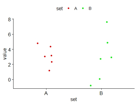
It can be seen in Figure 6.1 that, while values of data set A are grouped close to their mean, while the values of data set B are more spread out. We say that values of data set B are more dispersed (or scattered) than those of data set A. This example shows that the measures of central tendency are not enough in describing a set of data. In addition to using these measures, we need numerical measures of dispersion (or variation) of a set of data.
Dispersion refers to the extent to which numerical data values deviate from an average or central value. The statistical measures calculated from the data to quantify this dispersion are known as measures of dispersion.
6.1 Characteristics of a good measure of dispersion
An ideal measure of dispersion is expected to possess the following properties
It should be rigidly defined.
It should be based on all the items.
It should not be unduly affected by extreme items.
It should lend itself for algebraic manipulation.
It should be simple to understand and easy to calculate.
The most important measures of dispersion are range, quartile deviation, variance, inter-quartile range, mean absolute deviation and standard deviation.
6.2 The range
This is the simplest possible measure of dispersion. The range of a set of data is defined as the difference between the largest observation and the smallest observation in the set of data.
Thus,
Range = largest observation – smallest observation.
It can be denoted as, Range = L – S.
where, L = Largest value; S = Smallest value.
Example 6.1: The marks obtained by 8 students in mathematics and physics examinations are as follows:
| Student | Mathematics | Physics |
|---|---|---|
| 1 | 35 | 50 |
| 2 | 60 | 55 |
| 3 | 70 | 70 |
| 4 | 40 | 65 |
| 5 | 85 | 89 |
| 6 | 96 | 68 |
| 7 | 55 | 72 |
| 8 | 65 | 80 |
Find the ranges of the two sets of data. Are the physics marks more dispersed than the mathematics marks?
Solution 6.1
For mathematics,
Highest mark = 96, lowest mark = 35, range = 96 – 35 = 61
For physics,
Highest mark = 89, lowest mark = 50, range = 89 – 50 = 39.
The mathematics marks have a wider range than the physics marks. The mathematics marks are therefore more dispersed than the physics marks.
In individual observations and discrete series, L and S are easily identified. In case of grouped frequency distribution, the following method is employed.
L = Upper boundary of the highest class
S = Lower boundary of the lowest class.
\[Range = L - S \tag{6.1}\]
Example 6.2: Calculate range from the following distribution
| Size | 60–63 | 63–66 | 66–69 | 69–72 | 72–75 |
| Number | 5 | 18 | 42 | 27 | 8 |
Solution 6.2
L = Upper boundary of the highest class = 75
S = Lower boundary of the lowest class = 60
Range = L – S = 75 – 60 = 15
Merits and demerits of range
Merits
It is simple to understand.
It is easy to calculate.
In certain types of problems like quality control, weather forecasts, share price analysis, etc.
Demerits
It is very much affected by the extreme items.
It is based on only two extreme observations.
It cannot be calculated from open-end class intervals.
It is not suitable for mathematical treatment.
It is a very rarely used measure.
6.3 The inter-quartile range (IQR)
The range is a simple and quick measure to calculate. However, because it relies solely on the maximum and minimum values in a data set, it does not provide information about how the data is distributed between these two values. As a result, the range may not be an effective measure of dispersion, especially if one or both of these values are significantly different from the rest of the data. To address this limitation, the interquartile range is often used. The interquartile range is a more robust measure of dispersion, defined as the difference between the upper and lower quartiles of the data. IQR is also known as midspread. Thus,
\[IQR = Q_3 - Q_1 \tag{6.2}\]
The inter-quartile range of a set of data is therefore not affected by values of the data outside Q1 and Q3 making it a more reliable measure of spread for skewed or non-normal distributions.
Example 6.3: Consider the two sets of data A & B below, find IQR
| A | 3 | 4 | 5 | 6 | 8 | 9 | 10 | 12 | 15 |
| B | 3 | 8 | 8 | 9 | 9 | 9 | 10 | 10 | 15 |
For data set A, Q1 = 4.5, Q3 = 11; so Inter-Quartile Range = 11 – 4.5 = 6.5
For data set B, Q1 = 8, Q3 = 10; so Inter-Quartile Range = 10 – 8 = 2
Since the interquartile range (IQR) of data set A is greater than that of data set B, these results indicate that data set A is more dispersed than data set B. It is also noticeable that the range is the same for both sets.
Merits and demerits of IQR
Merits
It is simple to calculate and easy to understand.
It is not affected by extreme values (outliers) in the data, making it a more reliable measure of spread than the range.
IQR provides a clear measure of the spread of the middle 50% of the data, giving a better representation of variability when data is skewed.
It can be used for skewed distributions, where the range and standard deviation may not be as useful.
IQR is particularly useful in identifying outliers, as data points outside 1.5 times the IQR from the quartiles are often considered outliers.
Demerits
The IQR does not use all the data points, which means it may not represent the variability of the entire dataset.
It may not be as intuitive as the range or standard deviation for some users, particularly in more complex datasets.
The IQR is less sensitive to variations in the data outside of the interquartile range, meaning it might not fully reflect extreme values or trends.
It is not as effective when comparing datasets with significantly different shapes or distributions.
6.4 Mean absolute deviation (MAD)
The mean absolute deviation (MAD) is a measure of variability that indicates the average distance between observations and their mean. MAD uses the original units of the data, which simplifies interpretation. Larger values signify that the data points spread out further from the average. Conversely, lower values correspond to data points bunching closer to it. The mean absolute deviation is also known as the mean deviation and average absolute deviation.
Here is how to calculate the mean absolute deviation.
Calculate the mean.
Calculate the difference of each observation from mean and take absolute value i.e. ignore the sign. This difference is known as absolute deviation.
Add those deviations together.
Divide the sum by the number of data points.
\[MAD = \frac{\sum_{i = 1}^{n}\left| x_{i} - \overline{x} \right|}{n} \tag{6.3}\]
Example 6.4: Find the mean absolute deviation of the following 10, 15, 15, 17, 18, 21
| \[x_{i}\] | \[x_{i} - \overline{x}\] | \[\left| x_{i} - \overline{x}\right|\] |
|---|---|---|
| 10 | -6 | 6 |
| 15 | -1 | 1 |
| 15 | -1 | 1 |
| 17 | 1 | 1 |
| 18 | 2 | 2 |
| 21 | 5 | 5 |
| \(\overline{x} =\) 16 | \(\sum_{i = 1}^{n}\left| x_{i} - \overline{x} \right|\) = 16 |
Here n = 6 and \(\sum_{i = 1}^{n}\left| x_{i} - \overline{x} \right|\) = 16 therefore MAD = \(\frac{16}{6} = 2.67\)
Merits and demerits of MAD
Merits
Mean deviation is simple and easy.
Different items of observations can be easily compared with mean deviation.
Mean deviation is better than quartile deviation and range because it is based on all the observations of the series.
Mean deviation is less affected by the extreme values in the series while comparing to standard deviation.
Mean deviation is rigidly defined. So, it has fixed value.
Mean deviation about median will be least.
Demerits
Mean deviation becomes difficult to compute mean deviation in case of fractions.
It is not applicable for algebraic calculations.
It cannot be calculated from open-end class intervals.
Mean deviation is not a good measure as it ignores negative signs of deviations.
6.5 The variance and standard deviation
The most important measures of variability are the sample variance and the sample standard deviation. If x1, x2, …,xn is a sample of n observations, then the sample variance is denoted by s² and is defined by the equation.
\[ \mathbf{\text{sample variance}},\mathit{s}^{2} = \frac{\sum_{i = 1}^{n} (x_{i} - \overline{x})^{2}}{n - 1} \tag{6.4}\]
The sample standard deviation, s, is the positive square root of the sample variance.
\[\mathbf{\text{standard deviation} ,\mathit{s} = \ }\sqrt{\frac{\sum_{i = 1}^{n} (x_{i} - \overline{x})^{2}}{n - 1}} \tag{6.5}\]
Why standard deviation?
While both variance and standard deviation measure data dispersion, standard deviation is preferred for practical interpretation. Variance is expressed in squared units, making it harder to interpret. For example, if the data represents lengths in meters, the variance is in square meters (m²), which complicates understanding variability. In contrast, standard deviation is the square root of variance, preserving the original unit (e.g., meters), making it more intuitive. Thus, standard deviation is preferred for its clarity and ease of interpretation, especially when analyzing how data points deviate from the mean.
If the standard deviation of data set A is greater than that of data set B, it indicates that data set A is more dispersed than data set B. A higher standard deviation means that the values in data set A are more spread out from the mean compared to the values in data set B. It’s important to note that the standard deviation of any data set is always a non-negative number, as it represents the square root of the variance, which is always non-negative. Variance and standard deviation can never be negative values.
Example 6.5: Consider the Table 6.1 discussed earlier, find the standard deviation?
Solution 6.5
| Set A | \[x_{i}\] | \[x_{i} - \overline{x}\] | \[ \left( x_{i} - \overline{x} \right)^{2} \] |
| 1 | -2 | 4 | |
| 2 | -1 | 1 | |
| 3 | 0 | 0 | |
| 3 | 0 | 0 | |
| 4 | 1 | 1 | |
| 5 | 2 | 4 | |
| Sum | 18 | 0 | 10 |
Mean (\(\overline{x}\)) =\(\ \frac{18}{6} = 3\)
\[{Sample\ variance,\ s}_{A}^{2} = \frac{\sum_{i = 1}^{n}\left( x_{i} - \overline{x} \right)^{2}}{n - 1} = \frac{10}{5} = 2\]
\[\text{Sample standard deviation,}\ s_{A} = \ \sqrt{s_{A}^{2}} = \ \sqrt{2} = 1.414\]
| Set B | \[x_{i}\] | \[x_{i} - \overline{x}\] | \[ \left( x_{i} - \overline{x} \right)^{2} \] |
| -1 | -4 | 16 | |
| 0 | -3 | 9 | |
| 3 | 0 | 0 | |
| 3 | 0 | 0 | |
| 5 | 2 | 4 | |
| 8 | 5 | 25 | |
| Sum | 18 | 0 | 54 |
Mean (\(\overline{x}\)) =\(\ \frac{18}{6} = 3\)
\[{Sample\ variance,\ s}_{B}^{2} = \frac{\sum_{i = 1}^{n}\left( x_{i} - \overline{x} \right)^{2}}{n - 1} = \frac{54}{5} = 10.8\]
\[Sample\ standard\ deviation,\ s_{B} = \ \sqrt{s_{B}^{2}} = \ \sqrt{10.8} = 3.29\]
It can be seen that \(s_{B} > s_{A}\), confirming that data set B is more dispersed than data set A as shown in Figure 6.1.
An alternative formula for computing the variance
The computation of s² requires calculations of \(\overline{x}\), n subtractions and n squaring and adding operations. If the original observations or the deviations \(\left( x_{i} - \overline{x} \right)\) are not integers, the deviations \(\left( x_{i} - \overline{x} \right)\) may be difficult to work with, and several decimals may have to be carried to ensure numerical accuracy. A more efficient computational formula for s² is given by
\[s^{2} = \frac{1}{n - 1}\left\{ \sum_{i = 1}^{n}{x_{i}^{2} - \frac{1}{n}}\left( \sum_{i = 1}^{n}x_{i} \right)^{2} \right\} \tag{6.6}\]
Example 6.6: Consider the data set below; find standard deviation?
| 3 | 4 | 5 | 6 | 8 | 9 | 10 | 12 | 15 |
Solution 6.6
| \[x_{i}\] | \[x_{i}^{2}\] |
|---|---|
| 3 | 9 |
| 4 | 16 |
| 5 | 25 |
| 6 | 36 |
| 8 | 64 |
| 9 | 81 |
| 10 | 100 |
| 12 | 144 |
| 15 | 225 |
| \(\sum_{i=1}^{9} x_{i}\) = 72 | \(\sum_{i=1}^{9} x_{i}^{2}\) = 700 |
using Equation 6.6 ; here n = 9
\(s^{2} = \frac{1}{8}\left\{ 700 - {\frac{1}{9}\left( 72 \right)}^{2} \right\}\) = 15.5
\(s = \ \sqrt{15.5} = 3.94\)
6.5.1 Standard deviation for frequency table
For discrete frequency table
\[s^{2} = \frac{1}{n - 1}\left\{ \sum_{i = 1}^{n}{{f_{i}x}_{i}^{2} - \frac{1}{n}}\left( \sum_{i = 1}^{n}{f_{i}x}_{i} \right)^{2} \right\} \tag{6.7}\]
where, \(x_i\) is the ith observation and \(f_{i}\) is the corresponding frequency
Example 6.7: The frequency distributions of seed yield of 50 sesamum plants are given below. Find the standard deviation.
| Seed yield in gms (x) | 3 | 4 | 5 | 6 | 7 |
| Frequency (f) | 4 | 6 | 15 | 15 | 10 |
Solution 6.7
| \(x_{i}\) | \(f_{i}\) | \(f_{i}.x_{i}\) | \(f_{i}.x_{i}^{2}\) |
| 3 | 4 | 12 | 36 |
| 4 | 6 | 24 | 96 |
| 5 | 15 | 75 | 375 |
| 6 | 15 | 90 | 540 |
| 7 | 10 | 70 | 490 |
| Total | 50 | 271 | 1537 |
using Equation 6.7
\[{sample\ variance,\ s}^{2} = \frac{1}{50 - 1}\left\{ 1537 - \frac{271^{2}}{50} \right\} = 1.3914\]
\(standard\ deviation,\ s = \sqrt{1.3914}\) = 1.179
For grouped frequency table
\[s^{2} = \frac{1}{n - 1}\left\{ \sum_{i = 1}^{n}{{f_{i}d}_{i}^{2} - \frac{1}{n}}\left( \sum_{i = 1}^{n}{f_{i}d}_{i} \right)^{2} \right\} \tag{6.8}\]
where, \(f_{i}\) is the frequency of ith class, \(d_{i} = \frac{x_{i} - A}{c}\), where \(x_{i}\) is the class mark, \(A\) is the class mark with the highest frequency and c is the class interval.
Example 6.8: The frequency distributions of seed yield of 50 sesamum plants are given below. Find the standard deviation
| Seed yield in gms (x) | 2.5–3.5 | 3.5–4.5 | 4.5–5.5 | 5.5–6.5 | 6.5-7.5 |
| Frequency (f) | 4 | 6 | 15 | 15 | 10 |
Solution 6.8
Here n = 50; c = 1
| Seed yield | \(f_{i}\) | \(x_{i}\) | \[d_{i} = \frac{x_{i} - A}{c}\] | \(f_{i}.d_{i}\) | \(f_{i}.d_{i}^{2}\) |
|---|---|---|---|---|---|
| 2.5–3.5 | 4 | 3 | -2 | -8 | 16 |
| 3.5–4.5 | 6 | 4 | -1 | -6 | 6 |
| 4.5–5.5 | 15 | 5 | 0 | 0 | 0 |
| 5.5–6.5 | 15 | 6 | 1 | 15 | 15 |
| 6.5–7.5 | 10 | 7 | 2 | 20 | 40 |
| Total | 50 | 25 | 0 | 21 | 77 |
A = 5
using Equation 6.8
\[{sample\ variance,\ s}^{2} = \frac{1}{49}\left( 77 - \frac{\left( 21 \right)^{2}}{50} \right) = \ 1.3914\]
\(standard\ deviation,\ s = \sqrt{1.3914}\) = 1.179
6.5.2 Merits and demerits of standard deviation
Merits
It is rigidly defined and its value is always definite and based on all the observations.
As it is based on arithmetic mean, it has all the merits of arithmetic mean.
It is the most important and widely used measure of dispersion.
It is possible for further algebraic treatment.
It is less affected by the fluctuations of sampling and hence stable.
It is the basis for measuring the coefficient of correlation and other measures.
Demerits
It is not easy to understand and it is difficult to calculate.
It gives more weight to extreme values because the values are squared up.
As it is an absolute measure of variability, it cannot be used for the purpose of comparison.
6.6 Coefficient of variation
The standard deviation is an absolute measure of dispersion. It is expressed in terms of units in which the original figures are collected and stated. The standard deviation of heights of plants cannot be compared with the standard deviation of weights of the grains, as both are expressed in different units, i.e. heights in centimetre and weights in kilograms.
Therefore, the standard deviation must be converted into a relative measure of dispersion for the purpose of comparison. The relative measure is known as the coefficient of variation. The coefficient of variation is obtained by dividing the standard deviation by the mean and expressed in percentage.
\[\text{Coefficient of variation} \, (C.V) = \frac{\text{standard deviation}}{\text{mean}} \times 100 \tag{6.9}\]
A higher C.V. indicates greater variability in the dataset, meaning the data values are more dispersed relative to the mean. In contrast, a lower C.V. signifies lower variability, indicating that the data values are more closely clustered around the mean. This measure is particularly useful when comparing datasets with different units or scales.
Example 6.9: Consider the measurement on yield and plant height of a paddy variety. The mean and standard deviation for yield are 50 kg and 10 kg respectively. The mean and standard deviation for plant height are 55 cm and 5 cm respectively. Compare the variability.
Solution 6.9
Here, the measurements for yield and plant height are in different units. Hence the variability can be compared only by using coefficient of variation.
For yield, CV = \(\ \frac{10}{50} \times 100 =\) 20%
For plant height, CV = \(\frac{5}{55} \times 100 =\) 9.1%
The yield is subject to more variation than the plant height.
Exploring variability
The term “standard deviation” was first introduced in writing by Karl Pearson in 1894 in his paper “Contributions to the Mathematical Theory of Evolution.” Prior to this, the concept was referred to by other names, including “mean error,” “mean square error,” and “error of mean square,” reflecting its origins in the study of measurement errors and variability.(Pearson 1894)
The concept of variance was formalized in 1918 by Sir Ronald Aylmer Fisher in his seminal paper “The Correlation Between Relatives on the Supposition of Mendelian Inheritance.” While earlier mathematicians like Carl Friedrich Gauss made significant contributions to the development of probability and error theory, which influenced the understanding of variability, the term “variance” as we know it today was introduced by Fisher.(Fisher 1918)
“The object of our being statistical is to learn how to improve the whole health of humanity” – Florence nightingale