10 Probability
Probability is a cornerstone of statistical methods, providing the mathematical framework to quantify and analyze uncertainty. In the diverse and dynamic field of agricultural research, uncertainty often arises in areas such as yield predictions, pest control strategies, and the impact of environmental variables on crop growth. Understanding probability equips researchers and students with the tools to make informed decisions in the face of variability and randomness.
This chapter introduces fundamental probability concepts. We begin with the basic definitions and axioms of probability. The chapter progresses to explore key topics such as conditional probability, Bayes’ theorem, and independence of events.
10.1 Random experiment
A random experiment is a process or procedure that produces an outcome which cannot be predicted with certainty beforehand. The outcome is determined by chance, and the set of all possible outcomes is known as the sample space. Random experiments form the basis of probability theory and are critical for understanding uncertainty in various contexts.
Characteristics of a random experiment
Uncertainty of outcome: The result of the experiment cannot be predetermined.
Repeatability: The experiment can be repeated under the same conditions.
Defined sample space: All possible outcomes are known and well-defined.
Some common examples of random experiments used to illustrate probability theory were discussed below:
Tossing a coin
Tossing a coin is one of the simplest and most fundamental random experiments used to illustrate the principles of probability. Despite its simplicity, this seemingly mundane activity provides profound insights into random processes and lays the groundwork for understanding more complex probabilistic systems.
When a coin is tossed, there are two possible outcomes:
Heads (\(H\))
Tails (\(T\))
We say that for an unbiassed coin the probability of the coin landing \(H\) is \(\frac{1}{2}\) and the probability of the coin landing \(T\) is \(\frac{1}{2}\)
An unbiased coin is a theoretical concept in probability, referring to a coin designed or assumed to have no preference for either side when tossed, such that the likelihood of landing on heads (H) is exactly the same as landing on tails (T), with each outcome having a probability of \(\frac{1}{2}\) or 50%. Its characteristics include perfect symmetry, ensuring the coin is balanced without physical imperfections or uneven weight distribution that could influence the result, and equal probability, where each side is equally likely to face upward after a toss. This assumption generally holds under ideal experimental conditions, free from external factors like uneven surfaces or human bias in the tossing technique.
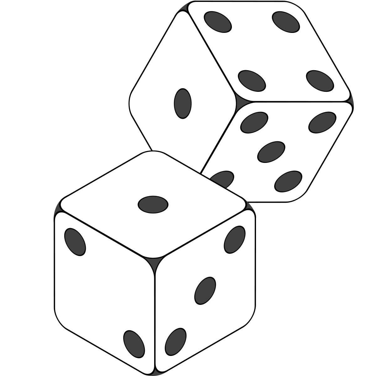
Throwing dice
A standard die has six faces, numbered from 1 to 6. Under fair conditions, each face has an equal probability of appearing when the die is rolled. Thus, the probability of getting any one face is \(\frac{1}{6}\).
Playing cards
A standard deck of playing cards consists of 52 cards, divided into four suits: spades, hearts, diamonds, and clubs, with each suit containing 13 cards. Four suits in playing cards were given in the Figure 10.2. The spades suit includes 9 numbered cards from 2 to 10, along with the picture cards ace, king, queen, and jack. Similarly, the hearts, diamonds, and clubs suits each contain 13 cards. Of these 52 cards, 26 are red, consisting of the hearts and diamonds suits, while the other 26 cards are black, comprising the spades and clubs suits. Playing cards can be used to create examples for random experiments, such as drawing a single card from a shuffled deck to determine its specific identity. Other experiments include drawing a card and checking its suit etc. These simple experiments can be easily modified with conditions or repetition, making playing cards a versatile tool for exploring probability and random events.


10.2 Random variable
A random variable is a numerical value that represents the outcome of a random experiment. It is a function that assigns a real number to each possible outcome in the sample space of the experiment.
Random variables can be classified into two types:
- Discrete random variables: These take on a countable set of values, such as integers (e.g., the number of heads in three coin tosses).
- Continuous random variables: These can take on any value within a given range, which is typically uncountable (e.g., the height of individuals in a population).
In mathematical terms, if \(S\) is the sample space of a random experiment, a random variable \(X\) is a function that maps sample space to real number set, which can be represented as \(X: S \to \mathbb{R}\), where \(\mathbb{R}\) represents the set of real numbers.
The probability of a random variable can be represented by \(p(X = x)\) or \(p(x)\), where the small letter \(x\) denotes the value taken by the random variable \(X\).
Consider the example of throwing a die once.Here, you can define a random variable of your interest. Defining a random variable involves assigning a numerical value to the outcomes of the experiment. Let \(X\) represent the number appearing on the die. The possible values of \(X\) are: \(x = \{1, 2, 3, 4, 5, 6\}\).
Consider another example of even number appearing on the die. Let \(X\) represent the even number appearing on the die. The possible values of \(X\) are: \(x = \{2, 4, 6\}\).
In each of the above case, you can see that the random variable \(X\) assigns a value to the outcomes of the experiment.
10.3 Probability
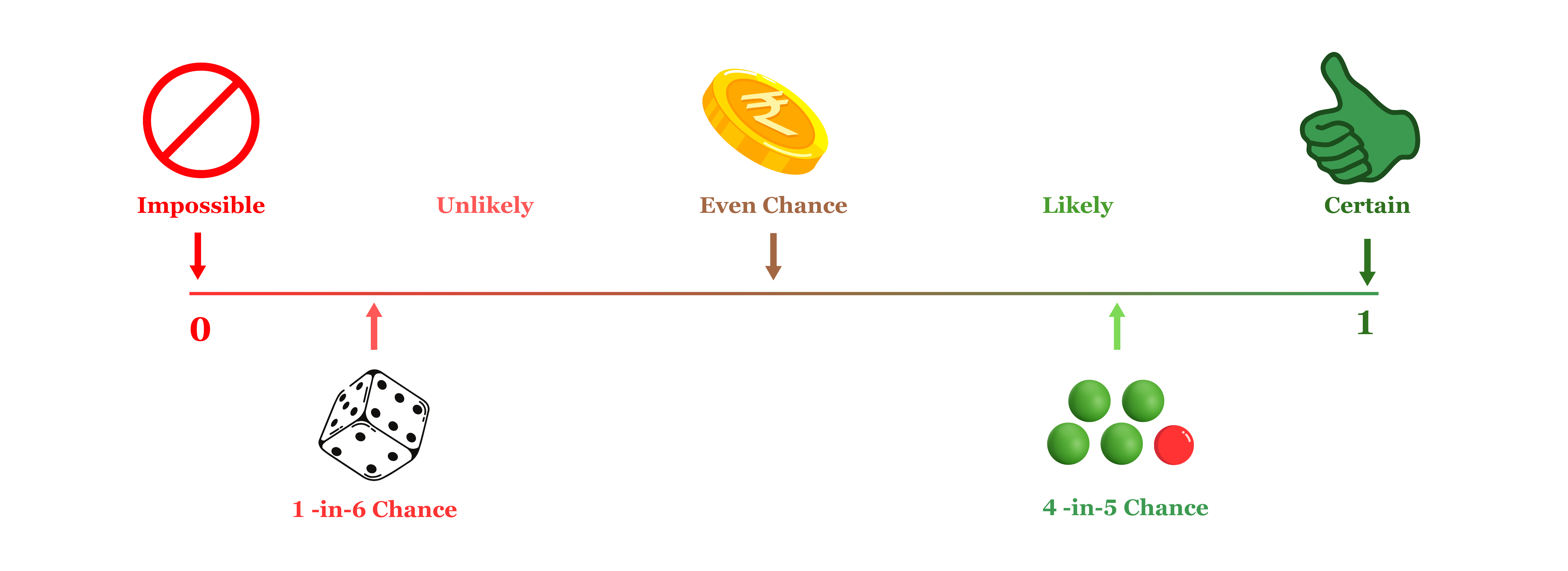
Probability is a measure of the likelihood or chance that a particular event will occur. It quantifies uncertainty and is expressed as a number between 0 and 1, where 0 indicates an impossible event and 1 represents a certain event. Mathematically, the probability of an event \(A\) is defined as the ratio of the number of favorable outcomes to the total number of possible outcomes, assuming all outcomes are equally likely, and is given by
Probability of an event \(A\) happening:
\[p(A) = \frac{\text{Number of favourable outcomes}}{\text{Total possible outcomes}} \tag{10.1}\]
here favourable outcome means outcomes favouring the happening of event \(A\).
Example 10.1: What is the chances of rolling a “4” with a die ?
Solution 10.1: Let the event \(A\) = rolling a “4” with a die. Number of ways event \(A\) can happen is one, as there is only 1 face with a “4” on it. Total number of outcomes is 6 (there are 6 faces altogether). So using Equation 10.1; probability,\(p(A)\) = \(\frac{1}{6}\).
Example 10.2: There are 5 marbles in a bag: 4 are blue, and 1 is red. What is the probability that a blue marble gets picked?
Solution 10.2: Let the event \(A\) = a blue marble gets picked. Number of ways event \(A\) can happen is 4 (there are 4 blues). Total number of possible outcomes is 5 (there are 5 marbles in total). So using Equation 10.1; probability,\(p(A)\) = \(\frac{4}{5}\) = 0.8
Common terms used
Outcome: An outcome is the result of a random experiment, representing a single occurrence or observation. For instance, when rolling a die, the outcomes could include the appearance of 1 dot, 2 dots, and so on.
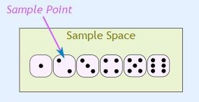
Sample space: The sample space (denoted as \(S\)) of a random experiment is the set that contains all possible outcomes of that experiment. For example, when tossing a coin, the sample space is \(S\) = {H, T}, and when throwing a die, the sample space is \(S\) = {1, 2, 3, 4, 5, 6}.
Sample point: A sample point is an individual element of the sample space, representing a single possible outcome. For example, “heads” in a coin toss or the “5 of clubs” in a deck of cards are sample points. In the case of rolling a die, there are six distinct sample points within the sample space.
Try yourself
If a die is tossed
- What is the sample space?
- What is the probability of getting a 1?
- What is the probability of obtaining a even number?
- What is the probability of getting a 7?
10.4 Event
An event refers to one or more outcomes of a random experiment. It can represent any subset of the sample space, where the event consists of specific outcomes that are of interest in the context of the experiment. An event can be a single outcome. For example, when tossing a coin, getting a “Tail” is an event that represents just one outcome from the sample space {H, T}. Similarly, rolling a “5” on a die is an event that includes only one specific outcome, 5, from the sample space {1, 2, 3, 4, 5, 6}.
On the other hand, an event can also include multiple outcomes. For instance, when selecting a “king” from a deck of cards, the event includes any one of the four kings (king of hearts, king of diamonds, king of clubs, king of spades), forming a set of four possible outcomes. Similarly, when rolling an “even number” on a die, the event would encompass the outcomes {2, 4, 6}, which are all the even numbers in the sample space of a die roll. Thus, an event can be a single outcome or a combination of multiple outcomes depending on the context of the experiment.
Example 10.3: Ram wants to see how many times a “double” (both dice have same number) comes up when throwing 2 dice.
Solution 10.3: The sample space is all possible outcomes (36 Sample Points): {1,1} {1,2} {1,3} {1,4} … {6,3} {6,4} {6,5} {6,6}. The event Ram is looking for is a “double”, where both dice have the same number. It is made up of these 6 sample points: {1,1} {2,2} {3,3} {4,4} {5,5} and {6,6}. You can calculate the probability of the event using Equation 10.1. Probability = \(\frac{6}{36}=0.17\).
10.4.1 Types of events
Independent events
Independent events are events where the occurrence of one does not influence the occurrence of another. For instance, consider tossing a coin. If it lands on “heads” three times in a row, the outcome of the next toss remains unaffected by the previous results. The probability of getting “heads” on the next toss is still \(\frac{1}{2}\) (or 0.5), just as it is for any fair coin toss. This demonstrates that past outcomes do not influence the probabilities of future events in independent scenarios.
Example 10.4: A coin is tossed 100 times, and heads appear in 99 of those tosses. What is the probability that heads will appear on the \(100^{th}\) toss?
Solution 10.4: Answer is \(\frac{1}{2}\) as each toss is independent of previous toss.
Dependent events
Dependent events are events where the outcome of one event influences the probabilities of subsequent events. For example, consider drawing cards from a deck. The probabilities change as cards are removed from the deck, altering the available outcomes. Initially, the chance of drawing a king on the first card is \(\frac{4}{52}\). However, for the second draw, the probabilities depend on the outcome of the first draw. If the first card is a king, only 3 kings remain among the 51 remaining cards, reducing the likelihood of drawing another king to \(\frac{3}{51}\). Conversely, if the first card is not a king, all 4 kings remain, making the probability \(\frac{4}{51}\). This illustrates how previous outcomes affect probabilities in dependent events.
When cards are drawn with replacement, each card is returned to the deck after being drawn, so the total number of cards remains constant. This keeps the probabilities unchanged, making the events independent. However, when cards are drawn without replacement, the total number of cards decreases after each draw, which alters the probabilities and makes the events dependent.
Mutually exclusive events
Mutually exclusive events are events that cannot occur at the same time. It is either one event or the other, but not both. For example, turning left or right is mutually exclusive because you cannot do both simultaneously. Similarly, heads and tails in a coin toss is mutually exclusive. Drawing a king and drawing an ace are mutually exclusive events because you can’t draw both in a single card. However, not all events are mutually exclusive. For instance, kings and hearts are not mutually exclusive because it is possible to have a king of hearts, an outcome that belongs to both categories.
Exhaustive events
A set of events is called exhaustive if, together, they encompass the entire sample space. For example, when tossing a die, the sample space is \(S = \{1, 2, 3, 4, 5, 6\}\). Consider the events: event \(A\), which is getting an even number \(\{2, 4, 6\}\), and event \(B\), which is getting an odd number \(\{1, 3, 5\}\). These events are exhaustive because, when combined, they include all possible outcomes in the sample space.
Equally likely events
Equally likely events are events that have the same theoretical probability of occurring. For example, when tossing a coin, event \(A\) (getting a head) and event \(B\) (getting a tail) are equally likely events because both have an equal probability of occurring.
10.5 Definitions of probability
In probability theory, different approaches are used to define and calculate the likelihood of events occurring. These approaches vary depending on the nature of the experiment and the available information. The three primary definitions of probability are mathematical (classical), statistical (empirical), and axiomatic, each offer unique perspectives and methods for determining probabilities. The classical approach is based on equally likely outcomes, the empirical approach relies on experimental data, and the axiomatic approach, developed by A.N. Kolmogorov, is based on a set of foundational principles. Understanding these definitions helps in applying probability theory to various real-world situations, from simple experiments to more complex scenarios.
10.5.1 Mathematical approach
It is also known as classical, theoretical or a priori approach to probability. If an experiment with \(n\) exhaustive, mutually exclusive and equally likely outcomes, \(m\) outcomes are favourable to the happening of an event \(E\), the probability \(p\) of happening of E is given by
\[p\left( E \right) = \ \frac{m}{n} \tag{10.2}\]
\(p\) is termed as probability of success.
Example 10.5: When a coin is tossed, there are two possible outcomes head or tail. Outcomes are exhaustive, mutually exclusive and equally likely. What is the probability of getting head?
Solution 10.5: Solution using mathematical approach, consider the event \(E\) : getting a head; probability of event \(E\), \(p(E)\) can be determined using Equation 10.2.
here, number of outcomes are favourable to the happening of event \(E\), \(m =1\); \(n\) = total number of possible outcomes (head and tail) = 2
\[p\left( E \right) = \ \frac{1}{2}\]
i.e. probability of getting a head is \(\frac{1}{2}\)
Limitations
The mathematical approach has certain limitations. For instance, it cannot account for situations where the outcomes are not equally likely, such as tossing a biased die. Additionally, this approach cannot define probability when the total number of possible outcomes \(n\) is unknown or tends to infinity, as in determining the probability of raining tomorrow. To address these limitations, other definitions of probability have been developed.
10.5.2 Statistical approach
The statistical approach to probability, also known as the empirical approach, is based on observing and recording outcomes from repeated experiments. The probability of an event is determined as the ratio of the number of times the event occurs \(m\) to the total number of trials \(n\) as when \(n\) approaches infinity. This method is useful when theoretical probabilities cannot be calculated but relies on the practicality of conducting a large number of trials and assumes consistency in experimental conditions.
The probability \(p\) of happening of \(E\) is given by
\[p\left( E \right) = \lim_{n \rightarrow \infty}\frac{m}{n} \tag{10.3}\]
where \(n\) is the number of times the process is performed which tends to infinity, and \(m\) is the number of times the outcome ‘\(E\)’ happens.
Limitations
The statistical approach also has limitations. In some cases, the experiment may not be practically repeatable, making it impossible to rely on repeated trials. Additionally, it raises the question of how large (\(n\)) must be to provide a good approximation of the probability. To address these issues, Russian mathematician A.N. Kolmogorov introduced the axiomatic approach, which does not rely on precise definitions but instead establishes probability based on a set of fundamental axioms or postulates.
10.5.3 Axiomatic Approach
The axiomatic approach to probability, introduced by A.N. Kolmogorov, provides a formal framework based on a set of foundational axioms rather than specific definitions. This approach overcomes the limitations of earlier methods by establishing universally accepted rules that apply to all probability calculations, making it applicable to a wide range of theoretical and practical scenarios.
Whole field of probability theory is based on the following three axioms
Probability of an event, \(p(E)\) lies between \(0\) and \(1\). That is \(0 \leq p(E) \leq 1\)
Probability of entire sample space is 1. That is \(p\left( S \right) = 1\)
If \(A\) and \(B\) are mutually exclusive events then probability of occurrence of either \(A\) or \(B\) is denoted by \(p(A \cup B)\) shall be given by \(p\left( A \cup B \right) = p\left( A \right) + p(B)\)
The probability \(p\) of the occurrence of an event is referred to as the probability of success, while the probability \(q\) of its non-occurrence is known as the probability of failure. Both \(p\) and \(q\) are non-negative and cannot exceed unity, i.e., \(0 \leq p \leq 1\) and \(0 \leq q \leq 1\). This means the probability of an event always lies between \(0\) and \(1\), inclusive. The probability of an impossible event is \(0\), and the probability of a certain event is \(1\). For instance, if \(p(A) = 1\), event \(A\) is guaranteed to occur, and if \(p(A) = 0\), event \(A\) cannot occur. Additionally, the number of favorable outcomes \(m\) for an event cannot exceed the total number of outcomes \(n\).
Example 10.6: In a simultaneous toss of two coins, find the probability of (i) getting 2 heads. (ii) exactly 1 head?
Solution 10.6: Here, the possible outcomes are HH, HT, TH, TT. i.e., Total number of possible outcomes = 4.
Number of outcomes favorable to the event (2 heads i.e.,HH) = 1. \(p\text{(2 heads)} = \frac{1}{4}\).
Now the event consisting of exactly one head has two favourable cases, namely HT and TH. \(p\text{(exactly one head)} = \frac{2}{4} = \frac{1}{2}\)
Example 10.7: In a single throw of two dice, what is the probability that the sum is 9?
Solution 10.7: The number of possible outcomes is 6 × 6 = 36.
(1,1) (1,2) (1,3) (1,4) (1,5) (1,6)
(2,1) (2,2) (2,3) (2,4) (2,5) (2,6)
(3,1) (3,2) (3,3) (3,4) (3,5) (3,6)
(4,1) (4,2) (4,3) (4,4) (4,5) (4,6)
(5,1) (5,2) (5,3) (5,4) (5,5) (5,6)
(6,1) (6,2) (6,3) (6,4) (6,5) (6,6)
Let the event \(A\) be sum the is 9. Four outcomes are there with sum 9, they are (5,4), (6,3), (3,6), (4,5). \(p (A) = \frac{4}{36} =\frac{1}{9}\)
Example 10.8: From a bag containing 10 red, 4 blue and 6 black balls, a ball is drawn at random. What is the probability of drawing (i) a red ball? (ii) a blue ball? (iii) not a black ball?
Solution 10.8: There are 20 balls in all. So, the total number of possible outcomes is 20
- Number of red balls = 10, \(p\text{(getting a red ball)}=\frac{10}{20} =\frac{1}{2}\)
- Number of blue balls = 4, \(p\text{(getting a blue ball)}=\frac{4}{20} =\frac{1}{5}\)
- Number of balls which are not black = 14, \(p\text{(not a black ball)}=\frac{14}{20} =\frac{7}{10}\)
10.6 Event relations
In probability theory, relationships between events help in analyzing their combined or individual outcomes within a sample space. These relations include concepts such as union, intersection, complement and mutual exclusivity, which are fundamental for understanding how events interact and influence probabilities.
Complement of an event
In probability, the complement of an event refers to all outcomes in the sample space that are not favorable to the given event. If \(A\) is an event, its complement is denoted by \(A^c\), and it represents the occurrence of all outcomes where \(A\) does not happen.
For example, consider the experiment of tossing a die. Let \(A\) be the event of getting an even number. The favorable outcomes for \(A\) are \(\{2, 4, 6\}\). The remaining outcomes, \(\{1, 3, 5\}\), do not satisfy \(A\) and are therefore the complement of \(A\). These outcomes represent the occurrence of \(A^c\), where \(A\) does not occur, therefore in this case \(A^c=\{1, 3, 5\}\) .
The complement of an event is essential in probability calculations and is related to the event by the formula:
\[P(A^c) = 1 - P(A) \tag{10.4}\]
The relationship in Equation 10.4 highlights that the probability of an event and its complement together always sum to 1. i.e. \(P(A) + P(A^c) = 1\)
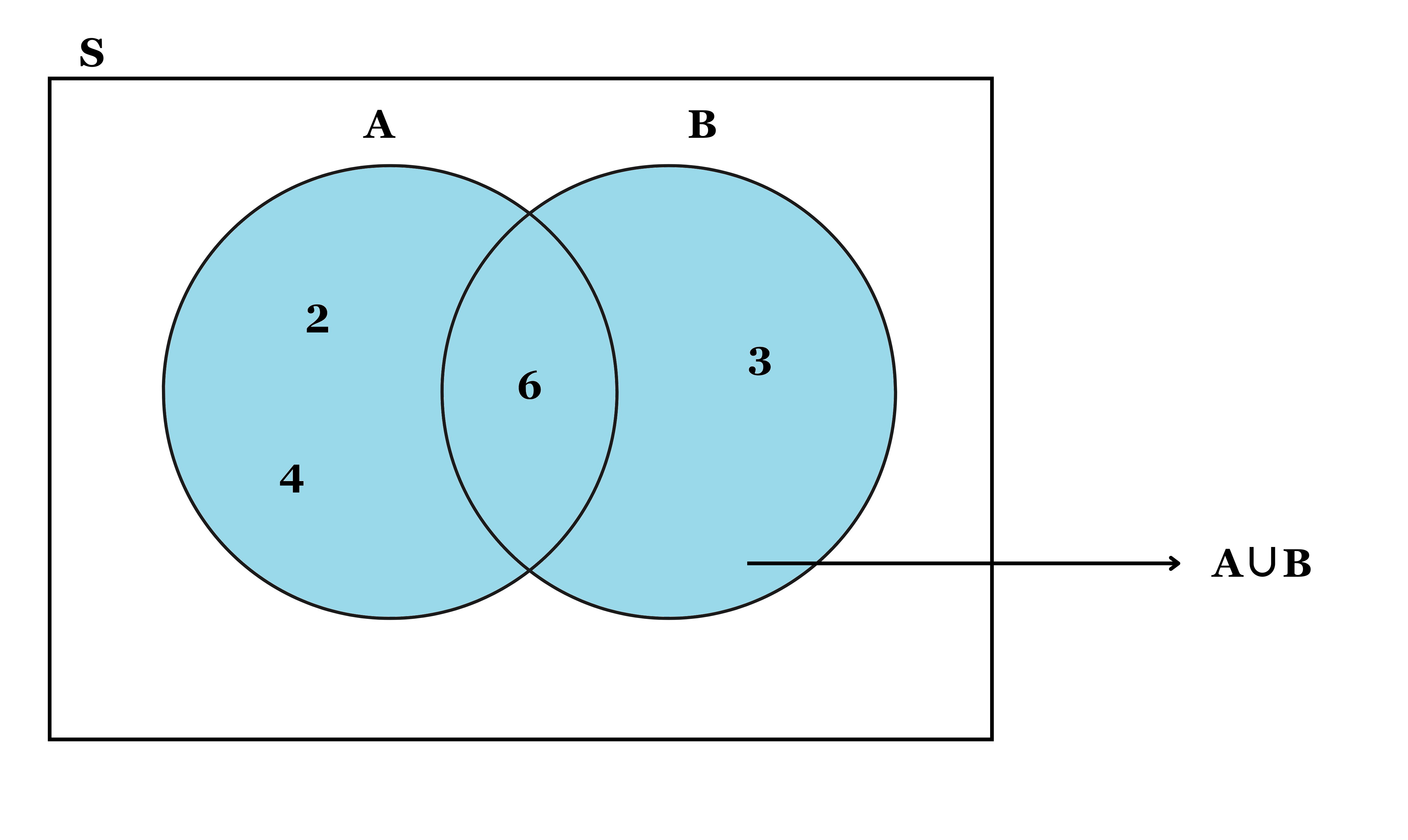
Event \(A\) or \(B\)
Denoted as ‘\(A \cup B\)’, spelled as \(A\) union \(B\), represents the occurrence of either event \(A\), event \(B\) or both. Let us consider the example of throwing a die. Suppose \(A\) is an event of getting a multiple of 2 and \(B\) be another event of getting a multiple of 3. The outcomes 2, 4 and 6 are favourable to the event \(A\) and the outcomes 3 and 6 are favourable to the event \(B\) i.e. \(A = \{2, 4, 6\}\), \(B= \{3, 6\}\) then \(A \cup B = \{ 2, 3, 4, 6\}\).
Event \(A\) and \(B\)
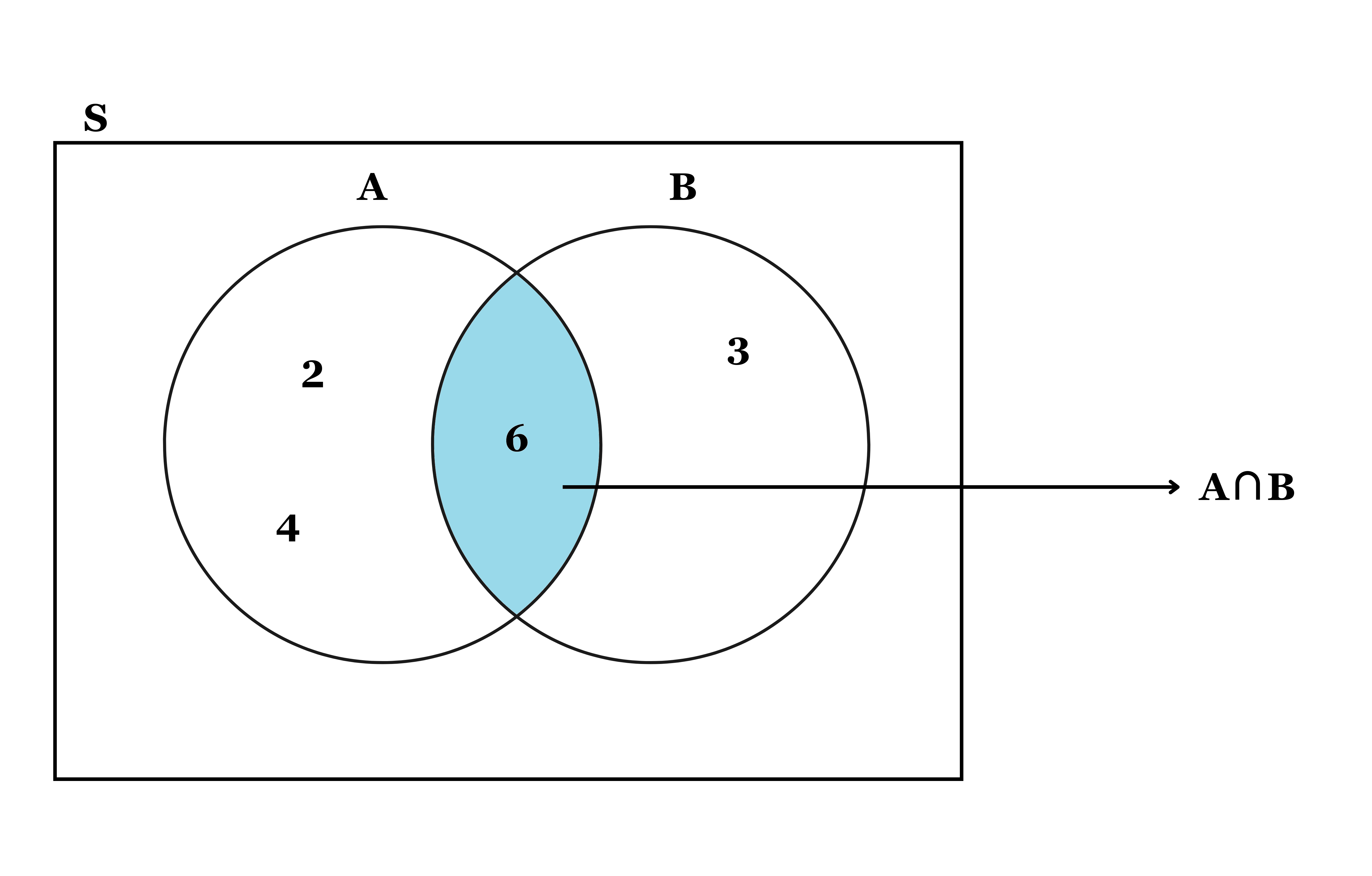
Denoted as ’ \(A \cap B\) ’ spelled as \(A\) intersection \(B\), represents the occurrence of both events \(A\) and \(B\) simultaneously. It includes only those outcomes that are common to both events. For example, on throwing a die in which \(A\) is the event of getting a multiple of 2 and \(B\) is the event of getting a multiple of 3. The outcomes favorable to \(A\) are 2, 4, 6 and the outcomes favorable to \(B\) are 3 and 6. Here 6 is present in both \(A\) and \(B\) so here \(A \cap B = 6\). Figure 10.6 below shows the venn diagram of intersection of two events.
10.7 Additive law of probability
According to additive law of probability, for any two events \(A\) and \(B\) of a sample space \(S\), the probability of the union of two events \(A\) and \(B\) is equal to the sum of their individual probabilities, minus the probability of their intersection.
\[p(A \cup B) = p(A)+p(B) − p(A \cap B) \tag{10.5}\]
For mutually exclusive case \(p(AꓵB)=0\); in that case:
\[p(A \cup B) = p(A )+ p(B ) \tag{10.6}\]
Example 10.9: A card is drawn from a well-shuffled deck of 52 cards. What is the probability that it is either a spade or a king?
Solution 10.9: If \(A\) denotes the event of drawing a ‘spade card’. \(B\) denotes the events of drawing a ‘king’ respectively. The event \(A\) consists of 13 sample points, whereas the event \(B\) consists of 4 sample points. \(p(A)= \frac{13}{52}\), \(p(B)= \frac{4}{52}\), \(p(A \cap B) = \frac{1}{52}\), \(p(A \cup B) = p(A)+ p(B) − p(AꓵB)\) = \(\frac{13}{52}+\frac{4}{52}-\frac{1}{52}= \frac{4}{13}\)
Example 10.10: In a single throw of two dice, find the probability of a total of 9 or 11.
Solution 10.10: Let the events \(A\) = a total of 9 and \(B\) = a total of 11. Events are mutually exclusive \(A \cap B = 0\). Now there are four such cases were sum = 9, such as (3, 6), (4, 5), (5, 4), (6, 3); therefore \(p(A) = \frac{4}{36}\). Similarly there are two cases were sum = 11, such as (5, 6), (6, 5); therefore \(p(B) = \frac{2}{36}\). Thus from Equation 10.6, \(p(A \cup B) = \frac{4}{36}+\frac{2}{36}= \frac{6}{36} = \frac{1}{6}\)
10.8 Conditional probability
Conditional probability measures the likelihood of an event occurring, given that another event has already occurred. If \(A\) and \(B\) are two events, the conditional probability of \(A\) given \(B\) is denoted by \(P(A \mid B)\) and is defined as:
\[p(A \mid B) = \frac{p(A \cap B)}{p(B)}, \quad \text{provided } p(B) > 0 \tag{10.7}\]
Equation 10.7 gives the probability of \(A\) happening under the condition that \(B\) has occurred.
Example 10.11: If a card is drawn from a standard deck of 52 cards, what is the probability that it is a king, given that the card drawn is a face card?
Solution 10.11: Let \(A\) be the event of drawing a king, \(B\) be the event of drawing a face card (king, queen, or jack). The probability of \(B\), drawing a face card, is \(p(B) = \frac{\text{Number of face cards}}{\text{Total cards}} = \frac{12}{52}\). The probability of \(A \cap B\), drawing a King that is also a face card, is:\(p(A \cap B) = \frac{\text{Number of Kings}}{\text{Total cards}} = \frac{4}{52}\). Using Equation 10.7 the conditional probability of drawing a king given that the card is a face card is \(p(A \mid B) = \frac{P(A \cap B)}{P(B)} = \frac{\frac{4}{52}}{\frac{12}{52}} = \frac{4}{12} = \frac{1}{3}\).
10.9 Multiplication law of probability
The multiplication law of probability states that if \(A\) and \(B\) are two events, the probability of both events occurring (i.e., \(A \cap B\)) is given by:
\[p(A \cap B) = p(A) \cdot p(B \mid A) \tag{10.8}\]
This formula expresses the relationship between the joint probability of two events and their conditional probability. If \(A\) and \(B\) are independent events, then \(p(B \mid A) = p(B)\), and the formula simplifies to:
\[p(A \cap B) = p(A) \cdot p(B) \tag{10.9}\]
Example 10.12: What is the probability of drawing two aces in succession from a standard deck of 52 cards?
Solution 10.12: Let \(A\) be the event that the first card drawn is an ace. \(B\) be the event that the second card drawn is an ace. The probability of \(A\) (drawing an ace on the first draw) is \(p(A) = \frac{4}{52}\). If the first card is an ace, there are only 3 aces left in a deck of 51 cards. The probability of \(B\) (drawing an ace on the second draw given that the first card was an ace) is \(p(B \mid A) = \frac{3}{51}\). Now using Equation 10.8 the probability of drawing two aces in succession is given by \(p(A \cap B) = p(A) \cdot p(B \mid A) = \frac{4}{52} \cdot \frac{3}{51} = \frac{12}{2652} = \frac{1}{221}\)
Example 10.13: A die is tossed twice. Find the probability of a number greater than 4 on each throw?
Solution 10.13: Let \(A\) be the event that ‘a number greater than 4’ on first throw. \(B\) be the event that ‘a number greater than 4’ in the second throw. Clearly \(A\) and \(B\) are independent events. In the first throw, there are two outcomes, namely, 5 and 6 favourable to the event \(A\). \(p(A) = \frac{2}{6} = \frac{1}{3}\). Similarly in the second throw, there are two outcomes, namely, 5 and 6 favourable to the event \(B\), therefore \(p(B) = \frac{2}{6} = \frac{1}{3}\). Now by Equation 10.6, probability to get a number greater than 4 on each throw is given by \(p(A \cap B) = p(A).p(B) = \frac{1}{3}.\frac{1}{3} = \frac{1}{9}\)
10.10 Probability using combinations
Combinations can be used to calculate the total number of possible outcomes in a probability problem. The formula for combinations is given by:
\[^n C_r = \frac{n!}{r!(n - r)!} \tag{10.10}\]
Example 10.14: Calculate \(^3 C_2\)
Solution 10.14: \(^3 C_2 = \frac{3!}{2!(3 - 2)!} = \frac{3 \times 2 \times 1}{2 \times 1} = 3\)
Example 10.15: A bag contains 3 red, 6 white, and 7 blue balls. What is the probability that two balls drawn are white and blue?
Solution 10.15: Total number of balls = 3 + 6 + 7 = 16. The number of ways to draw 2 balls from 16 is given by \(^{16} C_2 =120\). The number of ways to draw one white ball from 6 white balls is \(^6 C_1=6\), and the number of ways to draw one blue ball from 7 blue balls is \(^7 C_1 =7\). Since the events are independent, the total number of favorable outcomes is \(^6 C_1 \times ^7 C_1 = 6 \times 7 = 42\). Thus, the required probability is:\(p(\text{one white and one blue}) = \frac{^6 C_1 \times ^7 C_1}{^{16} C_2} = \frac{42}{120} = \frac{7}{20}\)
Example 10.16: A bag contains 5 red and 4 black balls. What is the probability that both balls drawn are red?
Solution 10.16:Total number of balls = 5 + 4 = 9. The number of ways to draw 2 balls from 9 is given by \(^9 C_2 = \frac{9 \times 8}{2 \times 1} = 36\). The number of ways to draw 2 red balls from 5 red balls is \(^5 C_2 = \frac{5 \times 4}{2 \times 1} = 10\). Thus, the required probability is: \(p(\text{both red balls}) = \frac{^5 C_2}{^9 C_2} = \frac{10}{36} = \frac{5}{18}\)
10.11 Bayes’ theorem
Bayes’ theorem gives a mathematical rule for inverting conditional probabilities, allowing one to find the probability of a cause given its effect.
Let \(E_1, E_2, \dots, E_n\) be a set of events associated with a sample space \(S\), where all the events \(E_1, E_2,\dots, E_n\) have non-zero probability of occurrence and they form a partition of \(S\). Let \(A\) be any event associated with \(S\), then according to Bayes theorem,
\[p(E_i \mid A) =\frac{p(E_i) \cdot P(A \mid E_i)}{\sum_{k = 1}^{n}{p(E_k)}\cdot p(A \mid E_k)} \tag{10.11}\]
The following terminologies are commonly used when applying Bayes’ theorem:
Hypotheses: The events \(E_1, E_2, \dots, E_n\) are called the hypotheses.
Prior probability: The probability \(p(E_i)\) is considered the prior probability of hypothesis \(E_i\).
Posterior probability: The probability \(p(E_i \mid A)\) is considered the posterior probability of hypothesis \(E_i\).
For any two events \(A\) and \(B\), the formula for the Bayes theorem is given by:
\[p(A \mid B) =\frac{p(B\mid A)\cdot p(A)}{p(B)}, p(B)\neq 0 \tag{10.12}\]
Where \(p(A)\) and \(p(B)\) are the probabilities of events \(A\) and \(B\). \(p(A \mid B)\) is the probability of event \(A\) given \(B\). \(p(B \mid A)\) is the probability of event \(B\) given \(A\).
Example 10.17: A bag I contains 4 white and 6 black balls while another bag II contains 4 white and 3 black balls. One ball is drawn at random from one of the bags, and it is found to be black. Find the probability that it was drawn from bag I.
Solution 10.17: Let \(E_1\) be the event of choosing bag I, \(E_2\) the event of choosing bag II, and \(A\) be the event of drawing a black ball. \(p(E_1)=p(E_2)=\frac{1}{2}\). Also,probability of drawing a black ball from bag I is given by \(p(A \mid E_1) = \frac{6}{10}=\frac{3}{5}\). Probability of drawing a black ball from bag II \(p(A \mid E_2=)\frac{3}{7}\).
By using Bayes’ theorem, the probability of drawing a black ball from bag I out of two bags,
\[p(E_1 \mid A) =\frac{p(E_1) \cdot P(A \mid E_1)}{p(E_1) \cdot P(A \mid E_1)+p(E_2) \cdot P(A \mid E_2)}\]
\[= \frac{\frac{1}{2}\times \frac{3}{5}}{\frac{1}{2}\times \frac{3}{5}+\frac{1}{2}\times \frac{3}{7}} =\frac{7}{12}\]
Example 10.18: A man is known to speak the truth 2 out of 3 times. He throws a die and reports that the number obtained is a four. Find the probability that the number obtained is actually a four.
Solution 10.18: Let \(A\) be the event that the man reports that number four is obtained. Let \(E_1\) be the event that four is obtained and \(E_2\) be its complementary event. Then, \(p(E_1)\) = probability that four occurs = \(\frac{1}{6}\). \(p(E_2)\) = probability that four does not occur = \(1-p(E_1) = 1-\frac{1}{6} = \frac{5}{6}\). Also, \(p(A|E_1)=\) probability that man reports four and it is actually a four \(= \frac{2}{3}\) (because man speaks truth 2 out of 3 times). \(p(A|E_2)=\)Probability that man reports four and it is not a four \(= \frac{1}{3}\).
By using Bayes’ theorem, probability that number obtained is actually a four, \(p(E_1 \mid A) =\frac{p(E_1) \cdot P(A \mid E_1)}{p(E_1) \cdot P(A \mid E_1)+p(E_2) \cdot P(A \mid E_2)}\).
\[p(E_1 \mid A)= \frac{\frac{1}{6}\times \frac{2}{3}}{\frac{1}{6}\times \frac{2}{3}+\frac{5}{6}\times \frac{1}{3}} =\frac{2}{7}\]
Try yourself
Six cards are drawn at random from a pack of 52 cards. What is the probability that 3 will be red and 3 black?
The gambler’s fallacy
In 1913, a group of gamblers gathered at a casino in Monte Carlo, where they witnessed a highly unusual event at the roulette table. The ball landed on black 26 times in a row—an incredibly rare streak. As the streak continued, more and more gamblers bet heavily on red, convinced that red was “due” to appear. But to their shock, black kept winning, and many lost fortunes that night. This event is now a famous example of the gambler’s fallacy also known as the Monte Carlo fallacy or the fallacy of the maturity of chances, the mistaken belief that past events influence future outcomes in independent events, like the spin of a roulette wheel. In reality, the probability of the ball landing on black or red remains the same on every spin, regardless of previous results.
“The theory of probabilities is at bottom nothing but common sense reduced to calculus.” – Pierre-Simon Laplace