11 Probability distributions
In statistics, a probability distribution gives the possibility of each possible outcome of a random experiment or event. It provides a systematic way to understand and quantify the probabilities of different occurrences.
Probability, as a measure of uncertainty, helps us analyze various phenomena. For instance, when rolling a die, the possible outcomes and their likelihoods are described by a probability distribution. Such distributions apply to any random experiment where outcomes are uncertain or unpredictable.
In this chapter, we explore the definition, functions, formulas, and types of probability distributions.
11.1 Probability distribution
In simple terms, a probability distribution is a way to represent all possible outcomes of a random variable, along with their corresponding probabilities. To understand this better, let us consider a random experiment—tossing an unbiased coin three times. Let \(X\) represent the number of heads that appear in these tosses. The possible outcomes for \(X\) are 0 heads, 1 head, 2 heads, and 3 heads, forming the sample space \(X = \{0, 1, 2, 3\}\). However, these outcomes are not equally likely. The total number of possible outcomes when tossing the coin three times is 8, as shown in Table 11.1.
| On tossing thrice | No: of heads (\(X\)) |
|---|---|
| HHH | 3 |
| HHT | 2 |
| HTH | 2 |
| THH | 2 |
| HTT | 1 |
| THT | 1 |
| TTH | 1 |
| TTT | 0 |
\(P(X = x)\) = \(\frac{No: \ of \ times\ X\ takes\ value\ x}{8}\)
\(P(X = 3)\) = 1/8; \(P(X = 2)\) = 3/8; \(P(X = 1)\) = 3/8; \(P(X = 0)\) = 1/8
Table 11.2 below shows the probability distribution of the number of heads that appear on tossing a coin 3 times.
| \(X\) | \(P(x)\) |
|---|---|
| 0 | 1/8 |
| 1 | 3/8 |
| 2 | 3/8 |
| 3 | 1/8 |
This is an example of discrete probability distribution as \(X\) takes only discrete values. If \(X\) takes continuous values, it is termed as continuous probability distribution.
11.2 Expected value of a random variable
Expected value is exactly what you might think it means: the return you can expect for some kind of action. The expected value of a random variable is the long-run average value of repetitions of the same experiment it represents. For example, the expected value in rolling a six-sided die is 3.5, because each face (1 through 6) has an equal chance of 1/6, and when you multiply each number by its probability and sum them up like 1/6 + 2/6 + 3/6 + 4/6 + 5/6 + 6/6, then you get 21/6, which is 3.5. It’s the average you’d see over countless rolls, even though you can’t roll a 3.5! The expected value of a random variable \(X\) is denoted as \(E(X)\).
The formula for calculating the Expected Value of random variable where there are multiple probabilities is given for discrete and continuous in Equation 11.1 and Equation 11.2.
Discrete case {.underline}
\[E(X) = \sum_{i = 1}^{\infty}xP(x) \tag{11.1}\]
Continuous case {.underline}
\[E(X) = \int_{- \infty}^{\infty}{x P(x)\ \text{dx }};- \infty \leq x \leq \infty \tag{11.2}\]
here the random variable \(X\) lies between \({-\infty}\) and \({+\infty}\)
Example 11.1: Find Expected value of \(X\) of tossing a single unfair die
| x | 1.0 | 2.0 | 3.0 | 4.0 | 5.0 | 6.0 |
| p(x) | 0.1 | 0.1 | 0.1 | 0.1 | 0.1 | 0.5 |
Solution 11.1:
| xp(x) | 0.1 | 0.2 | 0.3 | 0.4 | 0.5 | 3 |
Using equation Equation 11.1, \(E(X)\) = \(\sum_{i = 1}^{6}xP(x)\) = 0.1+0.2+0.3+0.4+0.5+3 = 4.5
Example 11.2: Find E(X) in the following case (solve it yourself)
| \(x\) | \(P(x)\) |
|---|---|
| 0 | 1/8 |
| 1 | 3/8 |
| 2 | 3/8 |
| 3 | 1/8 |
11.3 Discrete probability distributions
A discrete probability distribution represents the probabilities of outcomes of a discrete random variable, which takes on a countable number of distinct values. For example, the number of heads when flipping a coin three times or the number of defective items in a batch are described by discrete distributions. Each possible outcome is assigned a specific probability, and the sum of these probabilities is always 1.
We have seen that a probability distribution lists all possible outcomes of a random variable along with their corresponding probabilities, often represented as a table. However, it is often more convenient to express the distribution as an equation. With such an equation, the probability corresponding to any given value of \(x\) can be calculated directly. Depending on the situation, various discrete probability distributions are used to model different scenarios. In this chapter, we will focus on the following discrete distributions.
Bernoulli distribution
Binomial distribution
Poisson distribution
Probability mass function
When a probability function is used to describe a discrete probability distribution, it is referred to as a probability mass function (commonly abbreviated as p.m.f). A probability mass function assigns a probability to each specific outcome of a discrete random variable. It is expressed as: \(P(x) = P(X = x)\). Here, \(X\) is the discrete random variable, and \(P(x)\) represents the probability of \(X\) taking the specific value \(x\). The function ensures that all probabilities are non-negative and sum to 1 across all possible outcomes of \(X\).
Properties of p.m.f
The probability of each outcome is always non-negative. For a discrete random variable \(X\) and its p.m.f, \(P(x) \geq 0 \quad \text{for all } x\)
The sum of the probabilities over all possible values of the random variable equals 1. That is:\(\sum_{x \in S} P(x) = 1\). where \(S\) is the sample space of (\(X\)), representing all possible values.
The p.m.f gives the exact probability for each specific value of the discrete random variable. For a value \(x:P(X = x) = P(x)\)
If a value \(x\) is not in the sample space \(S\), its probability is zero: \(P(x) = 0 \quad \text{for } x \notin S\)
The p.m.f is defined only for the discrete values in the sample space of the random variable \(X\). It does not apply to continuous ranges or non-discrete variables.
11.3.1 Bernoulli distribution
A Bernoulli distribution is a discrete probability distribution that applies to a random experiment with exactly two possible outcomes, commonly referred to as “success” and “failure.” For example, tossing a coin results in two outcomes, which the experimenter can label as success and failure based on their context. Success might be defined as getting a head and failure as getting a tail. The definition of success and failure is flexible and can be tailored by the experimenter to suit the specific scenario under study.
The probability mass function of the distribution is
\[P(X = x) = p^x (1 - p)^{1 - x} \tag{11.3}\]
in Equation 11.3 \(X\) takes only two values = 0,1. Where \(p\) is the probability of success and \(1-p\) is the probability of failure.
A parameter of a distribution is a fixed value that describes a key characteristic of the distribution. The parameter of a Bernoulli distribution is \(p\), which represents the probability of success in a single trial
The expected value for a random variable, \(X\), from a Bernoulli distribution is: E(\(X\)) = \(p\) and the variance of a Bernoulli random variable is: var(\(X\)) = \(p(1 - p)\).
Example 11.3: Find the probability assuming Bernoulli distribution of a biased coin where probability of success (getting head) \(p\) = 0.4
Solution 11.3: Let \(X\) be the random variable which takes value 0 on getting tail (failure) and takes value 1 on getting head (success). So using the equation Equation 11.3
\(P(X = 0) = (0.4)^0 (1-0.4)^1 = 0.6\)
\(P(X = 1) = (0.4)^1 (1-0.4)^0 =0.4\)
the distribution can be shown as below:
| \(x\) | \(P(x)\) |
|---|---|
| 0 | 0.6 |
| 1 | 0.4 |
A Bernoulli trial is one of the simplest experiments you can conduct in probability and statistics. It’s an experiment where you can have one of two possible outcomes. For example, “Yes” and “No” or “Heads” and “Tails.”
11.3.2 Binomial distribution
Binomial distribution can be thought of as simply the probability of a success or failure outcome in an experiment or survey that is repeated multiple times; i.e. a Binomial distribution happens, when a Bernoulli trial is repeated \(n\) number of times. The binomial is a type of distribution that has two possible outcomes (the prefix “bi” means two, or twice). For example, if you toss a coin 5 times and count the number of heads, that count, \(X\), follows a binomial distribution with \(n = 5\). In short, a single coin toss is a Bernoulli trial, but repeating it several times (more than once) turns it into a binomial experiment.
Binomial distributions must also meet the following three criteria:
The number of observations or trials (\(n\)) is fixed.
Each observation or trial is independent
The probability of success(\(p\)) is exactly the same from one trial to another
The probability mass function of the distribution is
\[P(x) = \binom{n}{x} p^x q^{n-x} = \frac{n!}{x!(n-x)!} p^x q^{n-x} \tag{11.4}\]
where x takes values = 0,1,2,…, \(n\)
\(n\)= number of trials
\(x\)= number of success desired
\(p\)= probability of getting a success in one trial
\(q\) = \(1-p\) = probability of getting a failure in one trial
In a binomial distribution, the parameters are \(n\), the number of independent trials, and \(p\), the probability of success in a single trial. If X follows a binomial distribution we denote \(X \sim \text{Bin}(n, p)\). The mean of \(X\) is given by \(E(X) = np\), while the variance is \(\text{Var}(X) = npq\), where\(q = 1 - p\). Since \(0 < p < 1\), it follows that \(q\) is also positive but less than 1. This implies that \(np > npq\), establishing the fundamental property that the mean of a binomial distribution is always greater than its variance.
Example 11.4: A coin is tossed 10 times. What is the probability of getting exactly 6 heads?
Solution 11.4: here, \(n = 10; x = 6; p = \frac{1}{2}; q = 1-p = \frac{1}{2}\)
We have to find \(p(X=6)\); using the Equation 11.4
\(p(X=6)=\left( \frac{1}{2} \right)^{6}\left( \frac{1}{2} \right)^{10 - 6} = 0.2050\)
11.3.3 Poisson distribution
The Poisson distribution, discovered by the French mathematician Siméon Denis Poisson (1781–1840), was developed to describe the number of times a gambler would win a rarely won game of chance over a large number of tries. As a discrete probability distribution, it specifically deals with rare events. One of its earliest applications was in studying the number of deaths caused by horse kicks in the Prussian army, demonstrating its usefulness in modeling infrequent occurrences over a given interval of time or space.
Other applications and examples where Poisson distribution is used
Pest incidence
Birth defects and genetic mutations
Rare diseases
Car accidents
Traffic flow and ideal gap distance
Number of typing errors on a page
Hairs found in McDonald’s hamburgers
Spread of an endangered animal in Africa
Failure of a machine in one month
A random variable \(X\) is said to follow a Poisson distribution; if it assumes non-negative values and its probability mass function is given by:
\[p\left( X = x \right) = \frac{e^{- \lambda}.\lambda^{x}}{x!} \tag{11.5}\]
where \(x\) = 0,1,2,… ., \(\infty\),
\(e\) = Is the base of the natural logarithm. It is a constant approximately equal to 2.71828.
\(\lambda\) : Average number of successes occurring in a given time interval or region in the Poisson distribution
The parameter of Poisson distribution is \(λ\). If X follows a Poisson distribution we denote \(X \sim \text{poisson}(\lambda)\). The mean and the variance of the Poisson distribution are both equal to \(\lambda\)
Example 11.5: The average number of homes sold by a Realty company is 2 homes per day. Assuming Poisson distribution what is the probability that exactly 3 homes will be sold tomorrow?
Solution 11.5: here \(\lambda = 2\); since 2 homes are sold per day, on average.\(x= 3\); since we want to find the probability that 3 homes will be sold tomorrow. Using Equation 11.5.
\(p(X=3)= \ \frac{{2.71828}^{- 2}{\ \times \ 2}^{3}}{3!}= 0.180\)
Example 11.6: If the random variable X follows a Poisson distribution with mean 3.4, find \(p(X = 6)\)
Example 11.7: The number of industrial injuries per working week in a particular factory is known to follow a Poisson distribution with mean 0.5. Find the probability that in a particular week there will be: (a) Less than 2 accidents (b) More than 2 accidents
Example 11.8: A company known on the past experience that 3% of the bulbs they produced are defective. Assuming Poisson distribution find the probability of getting the following in a sample of 100 bulbs. (a) No defective (b) 1 defective
11.4 Continuous probability distributions
If the random variable X is continuous, the corresponding probability distribution is termed as continuous probability distribution. There are several continuous distributions. Our discussion is limited to only Normal distribution.
Probability density function
When a mathematical function is used to describe a continuous probability distribution, it is referred to as a probability density function (commonly abbreviated as p.d.f). It describes how values of a continuous random variable are distributed. It gives the relative likelihood of a variable taking a particular value within a given range. The area under the pdf curve over an interval represents the probability that the variable falls within that range. However, unlike pmf for discrete variables, the pdf itself does not give the probability of a single value but rather the density of possible values.
11.4.1 Normal distribution
The name “normal distribution” comes from its historical use in describing many natural and social phenomena that appeared to follow a similar symmetric, bell-shaped pattern. The term “normal” was popularized by Karl Pearson in the early 20th century, though the distribution itself was first studied by Abraham de Moivre and later formalized by Carl Friedrich Gauss.
The distribution was initially called the Gaussian distribution, as Gauss used it to model errors in astronomical observations. However, statisticians and scientists noticed that this pattern frequently appeared in various real-world data, such as heights, IQ scores, and measurement errors. Because it was so common, it became known as the normal distribution, implying that it represents a “normal” or typical way data is distributed in many natural processes.
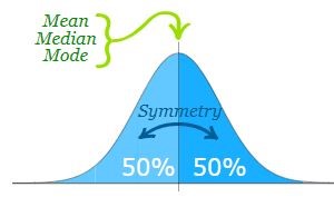
It is characterized by its symmetric, bell-shaped curve, where the mean, median, and mode are equal. Defined by two parameters, the mean (\(\mu\)) and standard deviation (\(\sigma\)). Its significance lies in the Central Limit Theorem, which states that the sum of a large number of independent random variables tends to be normally distributed, making it widely applicable in statistical inference. The normal distribution is defined by the following probability density function.
\[f\left( x \right) = \frac{1}{\sqrt{2\pi\sigma}}e^{- \frac{{(x - \mu)}^{2}}{2\sigma^{2}}} \tag{11.6}\]
, where \(- \infty < x < + \infty\) ; \(μ\) is the population mean and \(\sigma^2\) is the variance, \(e = 2.718\)
Parameters of Normal distribution
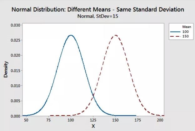
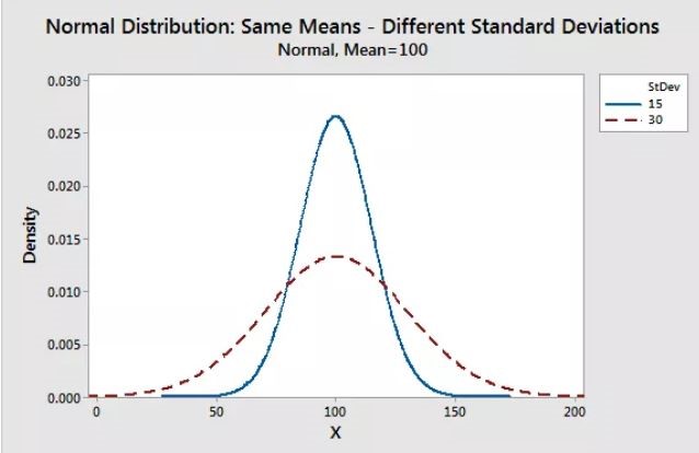
As with any probability distribution, the parameters of the normal distribution define its shape and probabilities entirely. The normal distribution has two parameters, mean (\(\mu\)) and standard deviation (\(\sigma\)). The normal distribution does not have just one form. Instead, the shape changes based on the parameter values.
Standard deviation:
The standard deviation is a measure of variability. It defines the width of the normal distribution. It determines how far away from the mean the values tend to fall. It represents the typical distance the observations and the average.
When you have normally distributed data, the standard deviation can be used to determine the proportion of the values that fall within a specified number of standard deviations from the mean. For example, in a normal distribution, 68% of the observation falls within \(\mu\pm \sigma\). This property is called as Area Property.
The parameters of normal distribution are \(\mu\) and \(\sigma\). If a random variable \(X\) follows the normal distribution, then we write \(X\sim\text{N}(\mu,\sigma^2)\). In particular, the normal distribution with \(\mu = 0\) and \(\sigma^2 =1\) is called the standard normal distribution, and is denoted as \(X\sim\text{N}(0,1)\)
Properties of Normal distribution
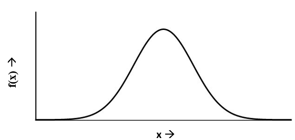
- The normal distribution is the most frequently used among all probability laws. The normal distribution can be found in many practical problems. If you plot density \(f(x)\) against \(x\) the graph will be bell shaped always.
- The Normal Distribution has mean = median = mode. Mean, median and mode is located to the center of the curve.
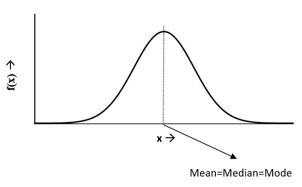
- Normal distribution is symmetric about the center, 50% of values less than the mean and 50% greater than the mean
- Area Property
The area property of the normal distribution shows how data is spread around the mean. As we move further from the mean, more values are included within the range. For example, about 68% of the data falls within one standard deviation of the mean. The area increases as we expand the range to two or three standard deviations, covering 95% and 99.7% of the data, respectively. See Table 11.6 for detailed information on the area property of the normal distribution.
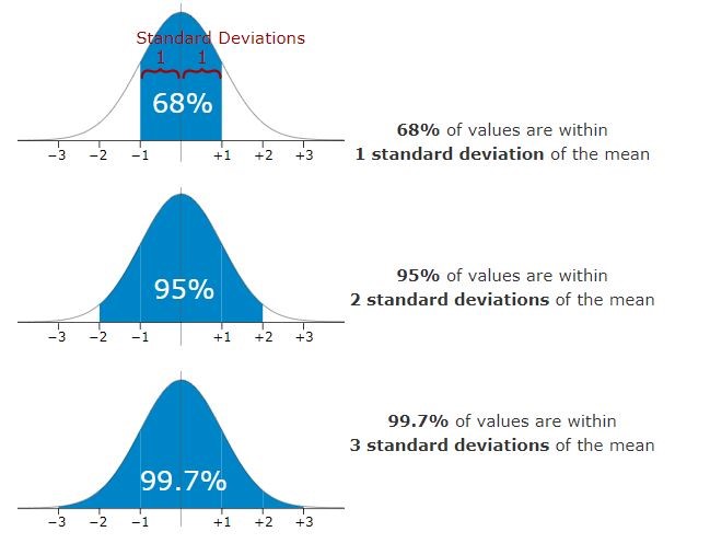
| Area | \(\%\) of value contained |
|---|---|
| \(\mu \pm 0.745\sigma\) | 50 |
| \(\mu \pm \sigma\) | 68.26 |
| \(\mu \pm 1.96\sigma\) | 95 |
| \(\mu \pm 2\sigma\) | 95.44 |
| \(\mu \pm 2.58\sigma\) | 99 |
| \(\mu \pm 3\sigma\) | 99.73 |
In short, a normal distribution is bell-shaped, symmetric, and has the property that the mean, median, and mode are all equal. It also has the area property. Other important properties of the normal distribution are listed below:
Defined by two parameters: The normal distribution is fully defined by its mean (\(\mu\)) and standard deviation (\(\sigma\)), where \(\mu\) determines the center and \(\sigma\) determines the spread or width of the curve.
Total area under the curve: The total area under the normal distribution curve is equal to 1, representing the total probability of all possible outcomes.
Asymptotic: The tails of the normal distribution approach, but never actually touch, the horizontal x-axis. This means the probability of extreme values is never exactly zero, but it becomes infinitesimally small.
Skewness and Kurtosis: A normal distribution has skewness equal to 0 (no skew), and kurtosis equal to 3 (mesokurtic), meaning it has a moderate peak and tails.
Linear combination: A linear combination of independent normal variables is also normally distributed. This property is crucial in statistical analysis and is a key reason for the widespread use of the normal distribution.
Central Limit Theorem: The normal distribution is central to the Central Limit Theorem, which states that the distribution of the sample mean will tend to be normal regardless of the shape of the original distribution, provided the sample size is sufficiently large.
Moments: All odd order moments are zero in normal distribution.
Dispersion: Quartile Deviation. Q.D = \(\frac{2}{3}\sigma\) and Mean Deviation. M.D = \(\frac{4}{5}\sigma\).
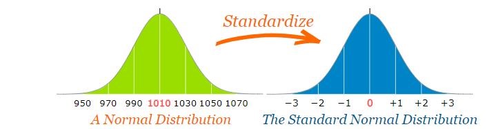
11.4.2 Standard Normal distribution
The standard normal distribution is a special case of the normal distribution where the mean is 0 and the standard deviation is 1. This distribution is also known as the Z-distribution. In the standard normal distribution, a value is referred to as a standard score or Z-score. The Z-score indicates how many standard deviations a data point is from the mean.
A normal distribution can be converted to a standard normal distribution, which provides several advantages:
- Simplifies calculations: With a mean of 0 and standard deviation of 1, performing statistical calculations becomes more straightforward.
- Universal comparison: Converting to a standard normal distribution allows comparison between different normal distributions on a common scale, regardless of their original means and standard deviations.
- Z-scores: The conversion enables the calculation of Z-scores, which measure the relative position of a data point in terms of standard deviations from the mean.
- Consistent analysis: It allows the use of standard normal distribution tables, making probability calculations more accessible and consistent across different datasets.
To convert a normal variate to a Standard Score (“z-score”)
First subtract the mean,
Then divide by the Standard Deviation
And doing that is called “Standardizing”.
When a normal variate $ X N(, ^2)$ is converted to a standard normal variate, it follows the transformation:
\[z = \frac{X - \mu}{\sigma} \tag{11.7}\]
Here, \(X\) is a normal variate with mean \(\mu\) and variance \(\sigma^2\), and \(z\) is the corresponding standard normal variate. This transformation converts \(X\) into a standard normal distribution \(z \sim N(0, 1)\), where the mean is 0 and the standard deviation is 1.
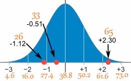
Example 11.6: A survey of daily travel time (\(X\)) had these results (in minutes): 26, 33, 65, 28, 34, 55, 25, 44, 50, 36, 26, 37, 43, 62, 35, 38, 45, 32, 28, 34. Convert it in to standard scores (Z-score).
Solution 11.6: The Mean (\(\mu\)) is 38.8 minutes, and the Standard Deviation (\(\sigma\)) is 11.4. Using Equation 11.7.
| \(X\) | \(X-\mu\) | \[z = \frac{X - \mu}{\sigma}\] |
|---|---|---|
| 26 | -12.8 | -1.12 |
| 33 | -5.8 | -0.51 |
| 65 | 26.2 | 2.30 |
| 28 | -10.8 | -0.95 |
| 34 | -4.8 | -0.42 |
| 55 | 16.2 | 1.42 |
| 25 | -13.8 | -1.21 |
| 44 | 5.2 | 0.46 |
| 50 | 11.2 | 0.98 |
| 36 | -2.8 | -0.25 |
| 26 | -12.8 | -1.12 |
| 37 | -1.8 | -0.16 |
| 43 | 4.2 | 0.37 |
| 62 | 23.2 | 2.04 |
| 35 | -3.8 | -0.33 |
| 38 | -0.8 | -0.07 |
| 45 | 6.2 | 0.54 |
| 32 | -6.8 | -0.60 |
| 28 | -10.8 | -0.95 |
| 34 | -4.8 | -0.42 |
Example 11.7: What is the z-score of a value of 27, given a set mean of 24, and a standard deviation of 2 ?
Solution 11.7: To find the z-score we need to divide the difference between the value, 27, and the mean, 24, by the standard deviation of the set, 2.\(z = \frac{27 - 24}{2} = \frac{3}{2} = 1.5\). This indicates that 27 is +1.5 standard deviations above the mean.
11.4.3 Z-Score Table
A Z-score table (or standard normal distribution table) shows the cumulative probability for a standard normal distribution, corresponding to different Z-scores. It provides the probability that a standard normal variable will be less than or equal to a given value. A model Z score table is given Figure 11.9.
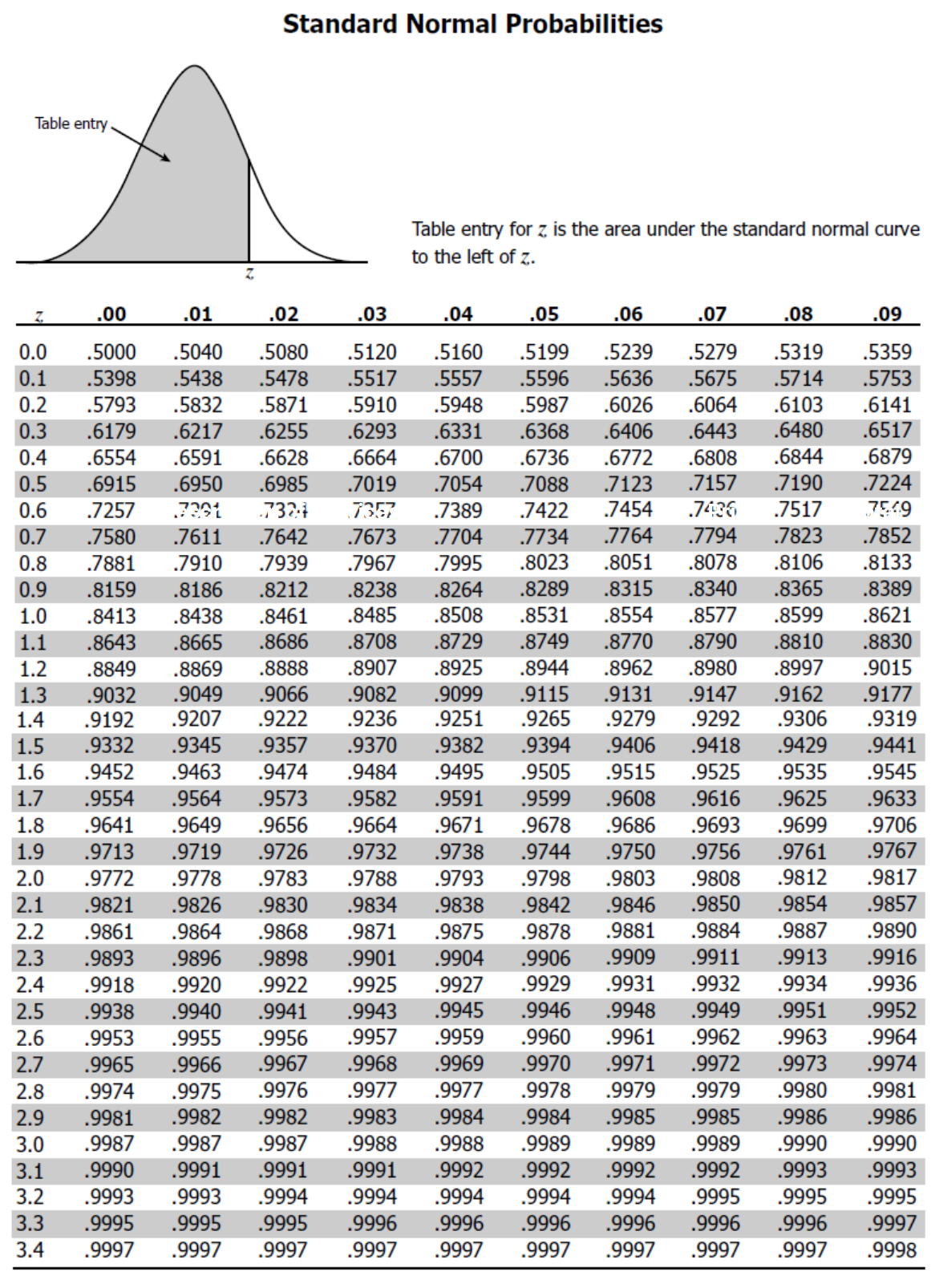
Procedure to use a Z-Score Table is given below:
Calculate the Z-score:
First, calculate the Z-score using the formula Equation 11.7Find the Z-score in the table:
Once you have the Z-score, locate its value in the Z-score table Figure 11.9. The table typically lists Z-scores in two parts: the first two digits (the ones and tenths place) are listed on the left, and the second decimal place is listed at the top. For example, for a Z-score of 1.23, find 1.2 on the left side and 0.03 across the top, and the value at the intersection is the cumulative probability.Interpret the table value:
The value from the Z-table represents the cumulative probability (area under the curve) to the left of the Z-score. For example A Z-score of 1.23 corresponds to a cumulative probability of about 0.8907, which means there is an 89.07% chance that a value from the distribution is less than or equal to 1.23 standard deviations above the mean.Use the table for finding areas:
To find the probability that a value lies above a certain Z-score, subtract the table value from 1. For example, if the Z-score is 1.23, the probability of a value being greater than 1.23 is: \(P(z > 1.23) = 1 - 0.8907 = 0.1093\). So, there is a 10.93% chance the value is above 1.23 standard deviations.For ranges of Z-scores:
If you’re looking for the probability that a value falls between two Z-scores, find the cumulative probabilities for both Z-scores and subtract the smaller from the larger. For example, for Z-scores of 1.23 and 0.5. From the table the cumulative probability for 1.23 is 0.8907. The cumulative probability for 0.5 is 0.6915. The probability that \(X\) lies between 0.5 and 1.23 is:\(P(0.5 < z < 1.23) = 0.8907 - 0.6915 = 0.1992\). By following these steps, you can use the Z-score table to find cumulative probabilities and interpret standard normal distribution data.
Example 11.8: Average yield of mango trees in an orchard has a mean of 70kg and with a standard deviation of 12kg. What is the probable percentage of mango trees with yield more than 85kg?
Solution 11.8: The z score for the given data using Equation 11.7 is \(z = \frac{85 - 70}{12}=1.25\). From the z score table Figure 11.9, the fraction of the data within this score is 0.8944. This means 89.44 % of the trees are within the yield of 85kg and hence the percentage of trees with yield above 85kg = (100-89.44)% = 10.56 %.
Example 11.9: The heights of coconut trees, H metres, are Normally distributed with a mean of 14.5 and a variance of 7 . Determine the probability that the height of a randomly chosen tree will be less than 12 metres.
Solution 11.9: Let H be the height of the tree. It is given that \(H \sim N(14.5,7)\). We nee to find \(P(H < 12)\). Which can be standardized to \(P(z < \frac{12 - 14.5}{\sqrt{7}})\)= \(P(z < -0.9442)\). Since normal distribution is symmetric, \(P(z < -0.9442)=P(z > 0.9442)\). \(P(z > 0.9442)= 1-P(z \leq 0.9442)\). From the table \(P(z \leq 0.95) =0.8289\) so the probability is 1-0.8289=0.171.
De Moivre’s Final Prediction
Abraham de Moivre, a French mathematician exiled to England, spent his life uncovering the hidden patterns of probability. Among his greatest contributions was the normal distribution, the elegant bell-shaped curve that governs everything from human traits to measurement errors. As he aged, de Moivre observed that his daily sleep was increasing by about 15 minutes, and in a striking prediction, he calculated that on the day his sleep reached 24 hours, he would die. Mysteriously, his forecast came true—he passed away on November 27, 1754. Though eerie, his work on probability lived on, later refined by Gauss and Laplace, shaping the foundation of modern statistics and proving that even randomness follows a predictable order.
“To understand God’s thoughts, we must study statistics, for these are the measure of his purpose.” — Florence Nightingale