7 Skewness and kurtosis
In the previous chapter, we explored numerical measures of central tendency and dispersion. Together, these measures give us insights into the location and spread of our data. However, they don’t fully describe the data distribution. What about its shape?
The shape of a distribution helps us understand the symmetry, peakedness, and presence of tails in the data. While a histogram provides a visual summary of the shape, we often need numerical measures for precise analysis. These measures include:
- Skewness, which quantifies the degree of asymmetry in the data distribution.
- Kurtosis, which measures the “tailedness” or peakedness of the distribution.
In this chapter, we will have a detailed discussion on these two important measures of shape, understanding how they are calculated and interpreted. By the end, you’ll be able to evaluate whether a distribution is symmetric, positively or negatively skewed, and whether it has light or heavy tails.
7.1 Skewness
Skewness is a measure of symmetry, or more precisely, the lack of symmetry. Then you may ask, what will a symmetric distribution looks like. Histogram of a symmetric distribution is showed in Figure 7.1.
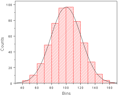
A distribution, or data set, is symmetric if it looks the same to the left and right of the centre point. In our discussion we are including only unimodal cases.
For a symmetric distribution skewness = 0; mean = median = mode. Figure 7.2 shows how a symmetric distribution looks like.
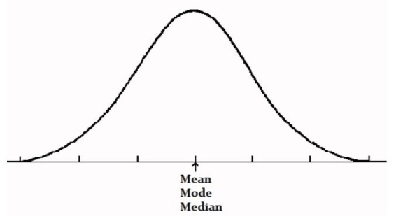
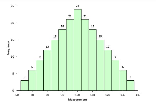
Figure 7.3 shows a model data set with skewness = 0 (symmetric distribution)
7.1.1 Negatively skewed
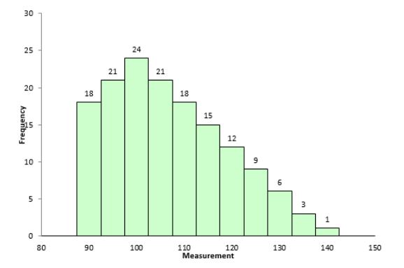
A negatively skewed distribution, also known as a left-skewed distribution, is characterized by a longer tail on the left side of the distribution. The bulk of the data values, or the “mass” of the distribution, is concentrated on the right, as shown in Figure 7.4.
This type of distribution is referred to as left-skewed, left-tailed, or skewed to the left because of the extended left tail. In such cases, the numerical relationship between the mean, median, and mode typically follows this pattern:
Mean < Median < Mode
This occurs because the mean is pulled towards the longer tail, while the median and mode remain closer to the center of the data’s bulk.
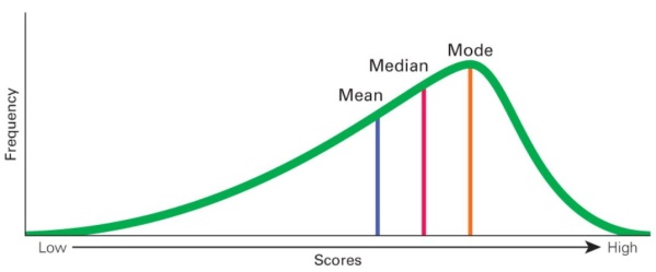
Figure 7.5 shows a model dataset with negative skewness.
7.1.2 Positively skewed
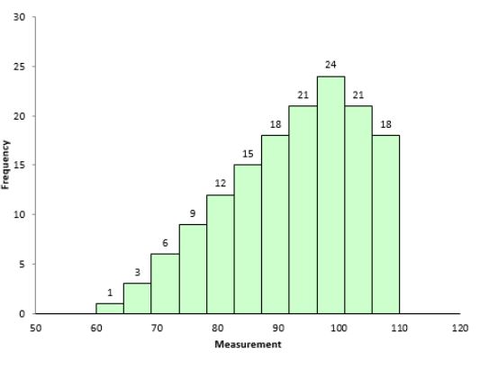
A positively skewed distribution, also known as a right-skewed distribution, is characterized by a longer tail on the right side. The bulk of the data values, or the “mass” of the distribution, is concentrated on the left, as illustrated in Figure 7.6.
This type of distribution is referred to as right-skewed, right-tailed, or skewed to the right, due to the extended tail on the right. In such cases, the relationship between the mean, median, and mode typically follows this pattern:
Mean > Median > Mode
This occurs because the mean is influenced by the extreme values in the longer right tail, while the median and mode remain closer to the center of the data’s bulk.
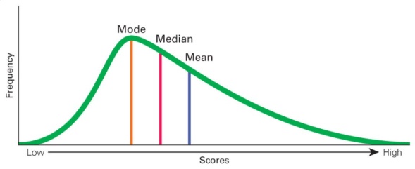
Figure 7.7 shows a model dataset with positive skewness.
7.2 Measures of skewness
The direction and extent of skewness can be measured in various ways. We shall discuss four measures.
7.2.1 Karl Pearson’s coefficient of skewness (\(S_{k}\))
You have noticed that the mean, median and mode are not equal in a skewed distribution. The Karl Pearson’s measure of skewness is based upon the divergence of mean from mode in a skewed distribution.
\[S_{k} = \frac{mean - mode}{\text{standard deviation}} \tag{7.1}\]
The sign of \(S_{k}\) gives the direction of skewness and its magnitude gives the extent of skewness. If \(S_{k}\) > 0, the distribution is positively skewed, and if \(S_{k}\) < 0 it is negatively skewed.
In Equation 7.1 since mode is used, there is a problem that if mode is not defined for a distribution we cannot find \(S_{k}\). But empirical relation between mean, median and mode states that, for a moderately symmetrical distribution \(\ mean - mode \approx 3(mean - median)\). So Equation 7.1 can be written as
\[S_{k} = \frac{3(mean - median)}{\text{standard deviation}} \tag{7.2}\]
Example 7.1: Compute the Karl Pearson’s coefficient of skewness from the following data:
| Height (x) | frequency (f) |
|---|---|
| 58 | 10 |
| 59 | 18 |
| 60 | 30 |
| 61 | 42 |
| 62 | 35 |
| 63 | 28 |
| 64 | 16 |
| 65 | 8 |
Solution 7.1
| Height (\(x_{i}\)) | frequency (\(f_{i}\)) | \(f_{i}x_{i}\) | \(f_{i}x_{i}^{2}\) |
|---|---|---|---|
| 58 | 10 | 580 | 33640 |
| 59 | 18 | 1062 | 62658 |
| 60 | 30 | 1800 | 108000 |
| 61 | 42 | 2562 | 156282 |
| 62 | 35 | 2170 | 134540 |
| 63 | 28 | 1764 | 111132 |
| 64 | 16 | 1024 | 65536 |
| 65 | 8 | 520 | 33800 |
| Sum | 187 | 11482 | 705588 |
Mean, \(\overline{x} = \frac{\sum_{i = 1}^{n}{f_{i}x_{i}}}{\sum_{i = 1}^{n}f_{i}}\) = \(\frac{11482}{187} = 61.40\)
\({Sample\ variance,\ s}^{2}\) using ?eq-sdfreq = \(\frac{705588 - \frac{\left( 11482 \right)^{2}}{187}}{186} = 3.123\)
\(Standard\ deviation,\ s = \sqrt{3.123} = 1.76\)
To calculate the median, refer to the Table 7.3. Locate the cumulative frequency just greater than \(\frac{n + 1}{2}\), and the corresponding value of \(x\) will be the median (\(Q_2\)).
Here, \(\frac{n + 1}{2} = \frac{187 + 1}{2} = \frac{188}{2} = 94\).
From the Table 7.3, it is evident that the median is 61.
| Height (\(x_{i}\)) | frequency (\(f_{i}\)) | cumulative frequency |
|---|---|---|
| 58 | 10 | 10 |
| 59 | 18 | 28 |
| 60 | 30 | 58 |
| 61 | 42 | 100 |
| 62 | 35 | 135 |
| 63 | 28 | 163 |
| 64 | 16 | 179 |
| 65 | 8 | 187 |
using Equation 7.2
\[S_{k} = \frac{3(61.40 - 61)}{1.76} = \frac{1.2}{1.76} = 0.68\]
Hence, the Karl Pearson’s coefficient of skewness \(S_{k}\) = \(0.68\), Thus the distribution is positively skewed.
7.2.2 Bowley’s measure of skewness (SQ)
Karl Pearson’s coefficient of skewness is most commonly used skewness measure. However, in order to use it you must know the mean, mode (or median) and standard deviation for your data. Sometimes you might not have that information; instead you might have information about quartiles. If that’s the case, you can use Bowley’s measure of skewness as an alternative to find out more about the asymmetry of your distribution. It’s very useful if you have extreme data values (outliers) or if you have an open-ended distribution.
\[{Bowley’s\ measure\ of\ Skewness,\ S}_{Q} = \frac{\left( Q_{3} - Q_{2} \right) - \left( Q_{2} - Q_{1} \right)}{\left( Q_{3} - Q_{2} \right) + \left( Q_{2} - Q_{1} \right)} \tag{7.3}\]
where, \(Q_{1}\) = 1st quartile; \(Q_{2}\) = median; \(Q_{3}\) = 3rd quartile
Equation can be further modified into
\[S_{Q} = \frac{Q_{3} - 2Q_{2} + Q_{1}}{Q_{3} - Q_{1}} \tag{7.4}\]
\(S_{Q}\) = 0 means that the curve is symmetrical.
\(S_{Q}\) > 0 means the curve is positively skewed.
\(S_{Q}\)< 0 means the curve is negatively skewed.
Lets find Bowley’s measure of skewness for Table 7.1 in Example 7.1 from the cumulative frequency in Table 7.3, quartiles can be calculated. Calculation of \({Q}_{1}\), \(Q_{2}\), \(Q_{3}\) is given in ?sec-quartile.
\[{Q}_{1} = 60\]
\[Q_{2} = 61\]
\[Q_{3} = 63\]
\[S_{Q} = \frac{63 - (2 \times 61) + 60}{63 - 60} = \ \frac{1}{3} = 0.33\]
Since \(S_{Q}\) > 0 means the curve is positively skewed.
7.2.3 Kelly’s measure of skewness (Sp)
Bowley’s measure of skewness is based on the middle 50% of the observations; it leaves 25% of the observations on each extreme of the distribution. As an improvement over Bowley’s measure, Kelly has suggested a measure based on Percentiles, including P10 and P90 so that only 10% of the observations on each extreme are ignored.
\[{Kelly's\ Measure\ of\ Skewness,\ S}_{p} = \frac{\left( P_{90} - P_{50} \right) - \left( P_{50} - P_{10} \right)}{\left( P_{90} - P_{50} \right) + \left( P_{50} - P_{10} \right)} \tag{7.5}\]
Try yourself
Try to find Kelly’s measure of skewness for Table 7.1
7.2.4 Measure based on moments
Before going into measuring skewness using moments, one should know what a moment is:
Moments
The rth moment about mean of a distribution, denoted by \(\mu_r\) is given by
\[\mu_{r} = \frac{\sum_{i = 1}^{N}{f_{i}\left( x_{i} - \overline{x} \right)^{r}}}{N} \tag{7.6}\]
where, \(f_{i}\) is the frequency of ith observation or class mark\(\ x_{i}\), \(N = \sum_{}^{}f_{i}\), number of observations
Moment about mean is also called as central moment.
If r = 0, \(\mu_{0} = \frac{\sum_{i = 1}^{N}{f_{i}\left( x_{i} - \overline{x} \right)^{0}}}{N}\) = 1
If r = 1, \(\mu_{1} = \frac{\sum_{i = 1}^{N}{f_{i}\left( x_{i} - \overline{x} \right)^{1}}}{N}\) = 0 (sum of deviation about mean is zero)
If r = 2, \(\mu_{2} = \frac{\sum_{i = 1}^{N}{f_{i}\left( x_{i} - \overline{x} \right)^{2}}}{N}\) = \(\sigma^{2}\), Population variance
It should be remembered that first moment about mean is 0 and second moment about mean is variance.
For Table 7.1 in Example 7.1 given above, calculate third central moment, \(\mu_{3}\)
| Height (\(x_{i}\)) | frequency (\(f_{i}\)) | \(\left( x_{i}-\overline{x} \right)^{3}\) | \({f_{i}\left( x_{i}-\overline{x}\right)}^{3}\) |
|---|---|---|---|
| 58 | 10 | -39.304 | -393.040 |
| 59 | 18 | -13.824 | -248.832 |
| 60 | 30 | -2.744 | -82.320 |
| 61 | 42 | -0.064 | -2.688 |
| 62 | 35 | 0.216 | 7.560 |
| 63 | 28 | 4.096 | 114.688 |
| 64 | 16 | 17.576 | 281.216 |
| 65 | 8 | 46.656 | 373.248 |
| Sum | 187 | 12.608 | 49.832 |
Mean = 61.40
\[\mu_{3} = \frac{\sum_{i = 1}^{N}{f_{i}\left( x_{i} - \overline{x} \right)^{3}}}{N} = \ \frac{49.832}{187} = 0.266\]
In short values of following moments about mean are
| Moments about mean | Value |
|---|---|
| \[\mu_{0}\] | 1 |
| \[\mu_{1}\] | 0 |
| \[\mu_{2}\] | \(\sigma^{2}\) |
Beta one and gamma one
The moment measure of skewness is based on the property that, for a symmetrical distribution, all odd ordered central moments are equal to zero. We note that \(\mu_{1}\) = 0, for every distribution, therefore, the lowest order moment that can provide an absolute measure of skewness is \(\mu_{3}\). So measures of skewness are based on \(\mu_{3}\).
\[\beta_{1} = \frac{\mu_{3}^{2}}{\mu_{2}^{3}} \tag{7.7}\]
Pronounced as ‘beta one’.
\(\beta_{1}\)= 0 means that the curve is symmetrical. The greater the value of \(\beta_{1}\) the more skewed the distribution. One serious limitation of \(\beta_{1}\) is that it cannot tell the direction of skewness i.e. whether it is positive or negative. Since \(\mu_{2}\) is always positive (as it is variance) and \(\mu_{3}^{2}\) is positive, \(\beta_{1}\) will be positive always. This drawback is removed by calculating \(\text{γ}_{1}\), called as Karl Pearson’s \(\text{γ}_{1}\), pronounced as ‘gamma one’.
\[\gamma_{1} = \sqrt{\beta_{1}} = \frac{\mu_{3}}{\mu_{2}^{3/2}} \tag{7.8}\]
If \(\mu_{3}\) is positive \(\gamma_{1}\) is positive, If \(\mu_{3}\) is negative \(\gamma_{1}\) is negative
\(\gamma_{1}\)= 0 means that the curve is symmetrical.
\(\gamma_{1}\) > 0 means the curve is positively skewed.
\(\gamma_{1}\)< 0 means the curve is negatively skewed.
For Table 7.1 in Example 7.1, \(\beta_{1}\) and \(\gamma_{1}\) can be calculated as follows
\(\mu_{3}\) = 0.226
\(\mu_{2}\) = 3.123
\(\beta_{1} = \frac{\mu_{3}^{2}}{\mu_{2}^{3}}\) = \(\frac{\left( 0.226 \right)^{2}}{\left( 3.123 \right)^{3}} = \ \frac{0.051}{30.46} = 0.0016\)
\(\gamma_{1} = \sqrt{\beta_{1}} = \ \sqrt{0.0016} = + 0.04\)
Since \(\mu_{3}\) is positive \(\gamma_{1}\)is positive. Since \(\gamma_{1}\) is slightly greater than 0, distribution is a slightly skewed to right.
7.3 Kurtosis
Kurtosis is a statistical measure that describes the shape of a distribution’s frequency curve, focusing on its relative peakedness. While skewness measures the asymmetry or lack of symmetry in a distribution, kurtosis evaluates how sharp or flat the peak of the curve is. There are three categories of frequency curves depending upon the shape of their peak as shown in Figure 7.8.
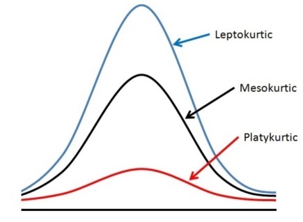
Kurtosis refers to degree of flatness or peakedness of the curve. It is measured relative to the peakedness of normal curve. The normal curve is considered as mesokurtic. If a curve is more peaked than normal curve, it is called leptokurtic. If a curve is more flat-topped than normal curve, it is called platykurtic. The condition of peakedness (leptokurtic) or flatness (platykurtic) is called kurtosis of excess.
7.3.1 Measure of kurtosis
Kurtosis is measured using \(\beta_{2}\) ‘beta two’ and \(\gamma_{2}\) ‘gamma two’ given by Karl Pearson
\[\beta_{2} = \frac{\mu_{4}}{\mu_{2}^{2}} \tag{7.9}\]
where, \(\mu_{4}\) is the 4th central moment, \(\mu_{2}\) is the 2nd central moment
\(\beta_{2}\) = 3 means that the curve is mesokurtic.
\(\beta_{2}\) > 3 means the curve is leptokurtic.
\(\beta_{2}\)< 3 means the curve is platykurtic.
\[\gamma_{2} = \beta_{2} - 3 \tag{7.10}\]
\(\gamma_{2}\) = 0 means that the curve is mesokurtic.
\(\gamma_{2}\) > 0 means the curve is leptokurtic.
\(\gamma_{2}\)< 0 means the curve is platykurtic.
For Table 7.1 in Example 7.1, kurtosis can be examined as follows
| Height (\(x_{i}\)) | frequency (\(f_{i}\)) | \(\left( x_{i}-\overline{x} \right)^{4}\) | \({f_{i}\left( x_{i}-\overline{x}\right)}^{4}\) |
|---|---|---|---|
| 58 | 10 | 133.634 | 1336.336 |
| 59 | 18 | 33.178 | 597.197 |
| 60 | 30 | 3.842 | 115.248 |
| 61 | 42 | 0.026 | 1.075 |
| 62 | 35 | 0.130 | 4.536 |
| 63 | 28 | 6.554 | 183.501 |
| 64 | 16 | 45.698 | 731.162 |
| 65 | 8 | 167.962 | 1343.693 |
| Sum | 187 | 391.021 | 4312.747 |
Mean, \(\overline{x}\) = 61.40
\(\mu_{2}\) = 3.123 (calculation shown in previous example)
\(\mu_{4} = \frac{\sum_{i = 1}^{N}{f_{i}\left( x_{i} - \overline{x} \right)^{4}}}{N} = \frac{4312.747}{187} = 23.062\)
\(\beta_{2} = \frac{\mu_{4}}{\mu_{2}^{2}} = \frac{23.062}{\left( 3.123 \right)^{2}} = 2.364\)
\(\beta_{2}\) is 2.364, which is close to 3, distribution can be considered slightly platykurtic close to symmetric.
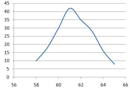
You can verify the frequency curve of Example 7.1 Figure 7.9, it can be seen that it is slightly right tailed (positively skewed).
“Crabs and kurtosis”
The story of kurtosis and skewness begins with a fascinating scientific journey involving crabs! In the late 1800s, Karl Pearson, a pioneering statistician, worked with biologist Walter Weldon to study variations in the size of crustaceans, like crabs. They noticed that the data didn’t follow the usual normal pattern, so Pearson developed new tools to better understand the shapes of these unusual data distributions.
He created the concept of skewness to measure whether the data was symmetrical or had long tails on one side. Then, he developed kurtosis, a measure of how “peaked” or “flat” the data distribution was compared to the normal curve. These ideas helped statisticians better analyze data that didn’t fit the typical patterns, paving the way for modern statistical tools we still use today! (Fiori and Zenga 2009)
“We are just statistics, born to consume resources” – Horace