2 Kruskal Wallis Test
Jithin Chandran1, Dr Pratheesh P Gopinath2
1Statoberry LLP, 2Department of Agricultural Statistics, Kerala Agricultural University,
The Kruskal-Wallis test is a non-parametric (distribution free) statistical test used to compare the medians of two or more independent groups when the data is not normally distributed or the assumptions of a one-way ANOVA are violated. It’s essentially a non-parametric equivalent of a one-way ANOVA, but instead of comparing means, it compares medians. It is named after William Kruskal and W. Allen Wallis, who developed it in 1952 (Kruskal and Wallis 1952).
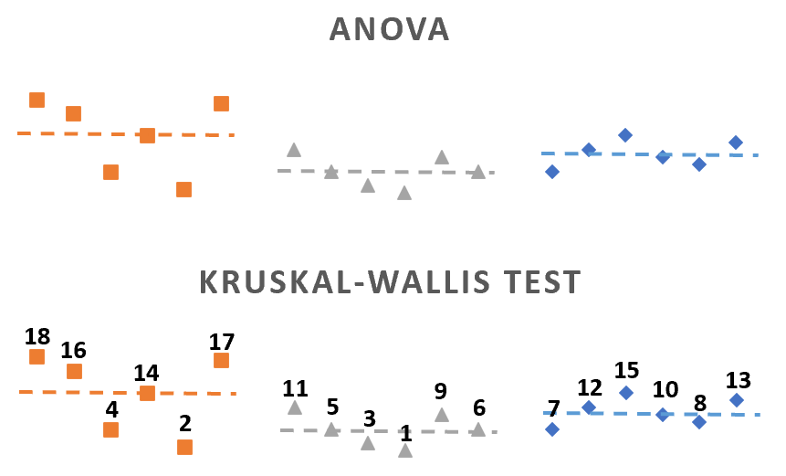
In the Kruskal Wallis test, it is enough for the data to be in the form of ordinal variables, which means values that can be ranked or ordered. This is because the test does not use the actual differences between the values. Unlike ANOVA, which compares group means using real quantitative values and assumes normal distribution and equal variances, the Kruskal Wallis test works by converting all observations into ranks and then checking how these ranks are distributed across the groups. This makes the Kruskal Wallis test suitable for situations where the data are not normally distributed or where the measurements are not precise but can still be ordered in a meaningful way. In the illustration in Figure 2.1, you can see ANOVA uses the actual data values, while the Kruskal Wallis test replaces them with their ranks to see if the groups are significantly different.
2.1 Example
Let’s explore some practical situations in agricultural research where the Kruskal-Wallis test, also known as the Kruskal-Wallis H test, is applied.
2.1.1 Study Context
- A food scientist is evaluating four drink flavours (V1 to V4) based on five sensory attributes: appearance, color, texture, taste, and flavour. Each flavour is rated by ten judges, so there are ten replications (ratings) per flavour. A Kruskal-Wallis test can be performed separately for each sensory attribute to check whether there are significant differences in ratings among the four flavours.Example1
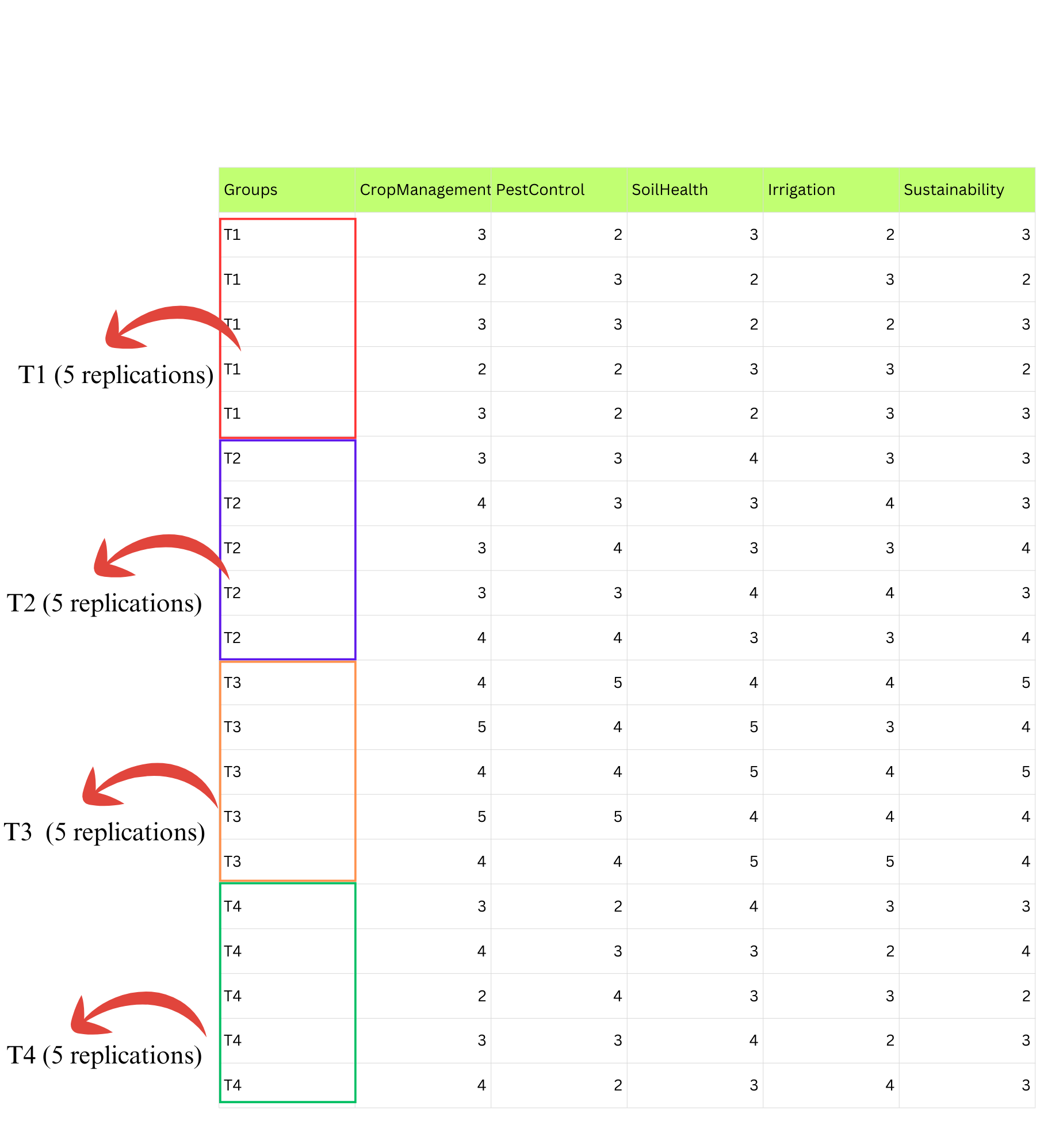
- An agricultural extension researcher is evaluating the effectiveness of four training methods (T1 to T4) based on how much knowledge farmers gain from each. Each method is tested on five different farmers, and their knowledge is scored after the training. Since each method is tested on five farmers, there are five replications per method. The Kruskal-Wallis test can be used to determine whether there is a significant difference in knowledge gain among the four training methods.Example2
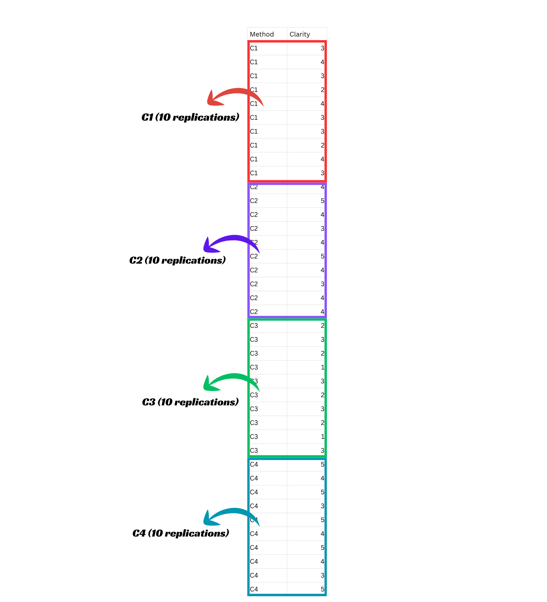
- An agricultural extension researcher is comparing four different communication methods (C1 to C4) for delivering farm advisories. Each method is tested on a separate group of 10 farmers, who rate the clarity of the information received. So, there are 10 farmers (or replications) for each method, making a total of 40 ratings. The Kruskal-Wallis test can be used to check whether there are significant differences in the clarity ratings among the four communication methods.Example3
2.2 Theory
You can either read through the theory of the Kruskal-Wallis test below, or, if you’re a non-statistician interested only in the practical aspects, you may skip ahead to Section 2.3, where we explain the test with a practical example. The theory section outlines the key steps involved in performing the Kruskal-Wallis test. Understanding these concepts will help you carry out the analysis with clarity and confidence.
2.2.1 Assumptions
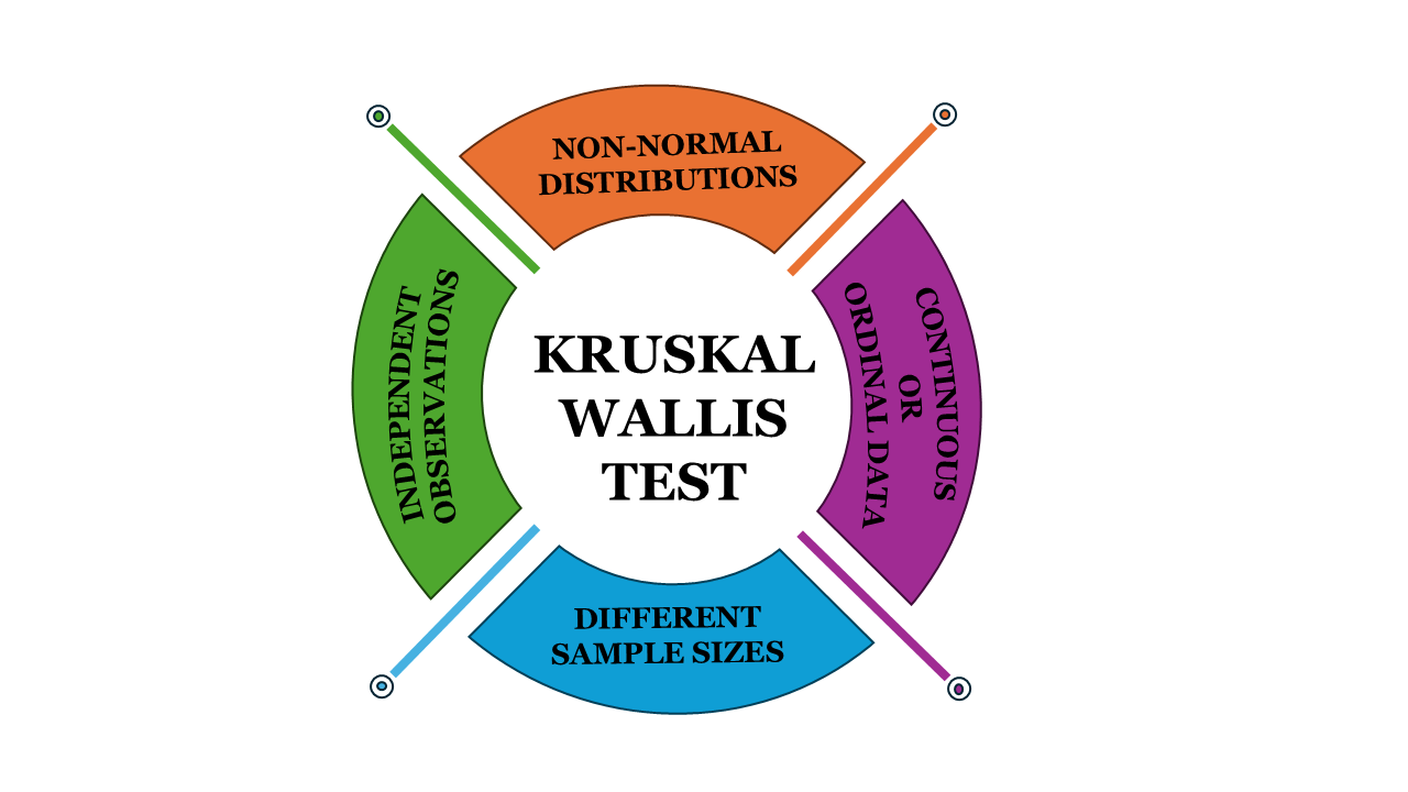
The Kruskal-Wallis test relies on the following assumptions:
Non-parametric: It does not assume a normal distribution of the data, making it suitable for non-normally distributed data
Independence of Observations: Each sample should be independent of the others, meaning there is no relationship or dependence between the observations within or across group
Ordinal or Continuous Data: The data can be ordinal, meaning it can be ranked, or continuous.
Key Features of Kruskal-Wallis Test
- Non-parametric: Unlike ANOVA, it does not assume normality or equal variances, making it suitable for non-normal data.
- Extension of the Mann-Whitney U test: It is essentially an extension of the Mann-Whitney U test, designed for more than two independent samples.
- Ranking-based: Like the Mann-Whitney U test, the Kruskal-Wallis test relies on ranking the data rather than using raw values.
- Test statistic: The test calculates a statistic based on the ranked data to determine if significant differences exist between the groups.
2.2.2 Hypotheses
The Kruskal-Wallis test evaluates the following hypotheses:
The population medians of all groups are equal.
At least one population median is different from the others.
Steps in Kruskal-Wallis Test
Step one: Sort and assign ranks to the data
Step two: Add up the ranks for each group
Step three: Calculate the H statistic
Step four: Obtain and interpret the p-value
2.2.3 The Test Statistic
The Kruskal-Wallis test statistic is calculated using the Equation 2.1
\[ \Large H = \frac{12}{N(N+1)} \sum_{i=1}^{k} \frac{R_i^2}{n_i} - 3(N+1) \tag{2.1}\] (Conover 1999)
Where:
- \(N\) is the total number of observations across all groups.
- \(k\) is the number of groups.
- \(n_i\) is the number of observations in group \(i\).
- \(R_i\) is the sum of ranks for group \(i\).
When there are no ties in the data, \(H\) follows a chi-square distribution with \(k-1\) degrees of freedom. When ties exist, a correction factor given in the Equation 2.2 is applied.
2.2.4 Correction for Ties
If there are tied values in the dataset, the test statistic is adjusted using:
\[ \Large H_{corrected} = \frac{H}{1 - \frac{\sum_{i=1}^{G} (t_i^3 - t_i)}{N^3 - N}} \tag{2.2}\]
Where:
- \(G\) is the number of groups of tied ranks.
- \(t_i\) is the number of tied values in the \(i\)-th group.
2.2.5 Interpreting the Results
The test statistic H approximately follows a chi-square distribution with k - 1 degrees of freedom, where k is the number of groups. To determine if the null hypothesis can be rejected, the H test value is compared to an H critical value obtained from a chi-square table by cross reference the degrees of freedom (df), with the level of significance (ɑ). If H exceeds the critical value, reject the null hypothesis
If you reject the null hypothesis, you can conclude that at least one group is significantly different from the others and proceed for multiple comparison tests.When the Kruskal-Wallis test shows a significant difference, it does not provide information about which specific pairs of groups are different. This is where post-hoc tests, like the Dunn test, become essential. They perform pairwise comparisons to identify exactly which groups differ, addressing the limitation of the Kruskal-Wallis test.
What is a post-hoc test?
A post-hoc test is a follow-up analysis performed after finding a significant result in an overall statistical test (like ANOVA or Kruskal-Wallis). Its purpose is to identify exactly which groups or treatments differ from each other. In other words, it helps pinpoint where the differences lie between multiple groups when the initial test shows that not all groups are the same.
2.2.6 Post-hoc test
When the Kruskal-Wallis test is significant, the following post hoc tests are commonly used for pairwise comparisons:
Dunn’s Test
The Dunn test is a post-hoc statistical procedure used in conjunction with the Kruskal-Wallis test. Used to determine which specific groups differ when the Kruskal-Wallis test indicates a significant difference among multiple groups. It compares the sums of ranks between every pair of groups by calculating the difference in their average ranks and standardizing this difference using an estimate of its standard error. The standardized test statistic in Dunn’s test is compared to the standard normal distribution (the Z-distribution) to determine significance. (Dunn 1964)
LSD (Least Significant Difference) Test
The nonparametric LSD test is a post-hoc procedure used after a significant Kruskal-Wallis test to find which groups differ. It calculates the minimum significant difference (MSD) between group mean ranks based on an estimate of rank variance and uses the Student’s t-distribution to determine significance. Groups are compared pairwise by checking if their mean rank differences exceed the MSD. This test assumes similar group sizes and equal variance of ranks, offering a simpler method to classify groups when these conditions hold.(Mendiburu 2020)
Which post-hoc test to use?
When choosing a post-hoc test after performing a Kruskal-Wallis test, the decision largely depends on the characteristics of your data and the goals of your analysis. Dunn’s test is the most commonly recommended method for nonparametric pairwise comparisons because it adjusts for multiple testing and compares standardized rank differences using the normal distribution, making it suitable for groups of unequal sizes and providing a more conservative control of Type I errors. On the other hand, the nonparametric LSD method, such as the one implemented in the agricolae package, is simpler and uses the Student’s t-distribution along with a minimum significant difference calculated on ranks. This method works well when group sizes are approximately equal and when ease of interpretation is preferred, although it tends to be less conservative and may lead to more false positives. Overall, Dunn’s test is generally preferred for its rigor and wider acceptance, while the nonparametric LSD can be a practical alternative in balanced designs, provided the results are interpreted with caution.
2.2.7 p Adjustment Method
In statistical hypothesis testing, p-values indicate the probability of observing results at least as extreme as those observed, assuming the null hypothesis is true. When multiple tests are conducted, the risk of false positives (Type I errors) increases. P-value adjustment methods address this issue by controlling the overall error rate, ensuring reliable inference in multiple testing scenarios.
Different p-adjustment methods are listed below, if you are interested you can click on them to read more:
- Bonferroni
- Holm
- Hommel
- Benjamini-Hochberg Procedure (BH)
- Benjamini-Yekutieli Procedure (BY)
- False Discovery Rate (q-value) Approach
Which p-adjustment method to use?
In agricultural research, it is a common practice to use no p-value adjustment (“none”) for multiple comparisons after tests like the Kruskal-Wallis. This is because agricultural experiments often involve smaller numbers of treatments and replications, where strict adjustments may be overly conservative and reduce the ability to detect meaningful differences. Researchers prefer to interpret results with caution rather than risk missing important findings due to overly strict error control. Nonetheless, the choice should always consider the study design, number of comparisons, and the consequences of Type I versus Type II errors in the specific context. However, When you have a large number of groups and sizable sample sizes, like in social science research, controlling the false discovery rate (FDR) becomes important to balance detecting true differences while limiting false positives. In such cases, the Benjamini-Hochberg (BH) procedure is often recommended. It controls the expected proportion of false discoveries (Type I errors) among the rejected hypotheses, which is less conservative than Bonferroni but still provides strong error control suitable for large-scale multiple testing. If your tests are dependent or more complex, the Benjamini-Yekutieli (BY) procedure can be used as it controls FDR under any dependency structure, though it is more conservative than BH.
2.3 Getting started in RAISINS
RAISINS (R and AI Solutions in INferential Statistics) is an online platform that simplifies data analysis for agricultural research. RAISINS is completely online and doesnot require any downloads. It integrates the power of R, Python, and AI to offer user-friendly, robust statistical tools. The platform is developed by STATOBERRY LLP, with mentorship from the Department of Agricultural Statistics, College of Agriculture, Vellayani, Kerala Agricultural University.
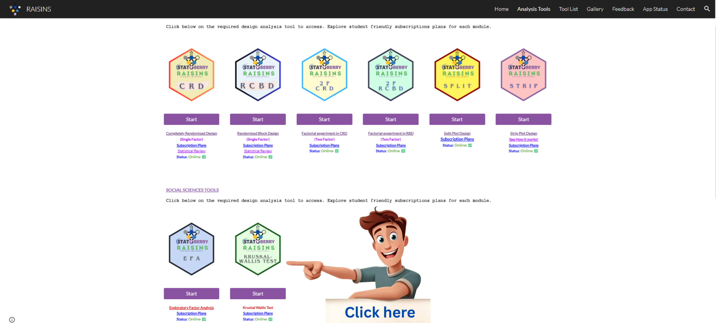
Head to www.raisins.live where you can access various analytical modules. You can accesss the kruskal wallis test module from the analysis tools under social science section
You can log in to the web application using the credentials you received after subscribing.
2.3.1 A working example
We’ll guide you through the entire Kruskal-Wallis test step by step. To begin, let’s look at how the analysis can be carried out using Example 1 described in Section 2.1.1. For clarity, here’s a quick recap of the example: A food scientist is evaluating four drink flavours (V1 to V4) based on five sensory attributes—appearance, color, texture, taste, and flavour. Each flavour is rated by ten judges, providing ten replications (ratings) per flavour.
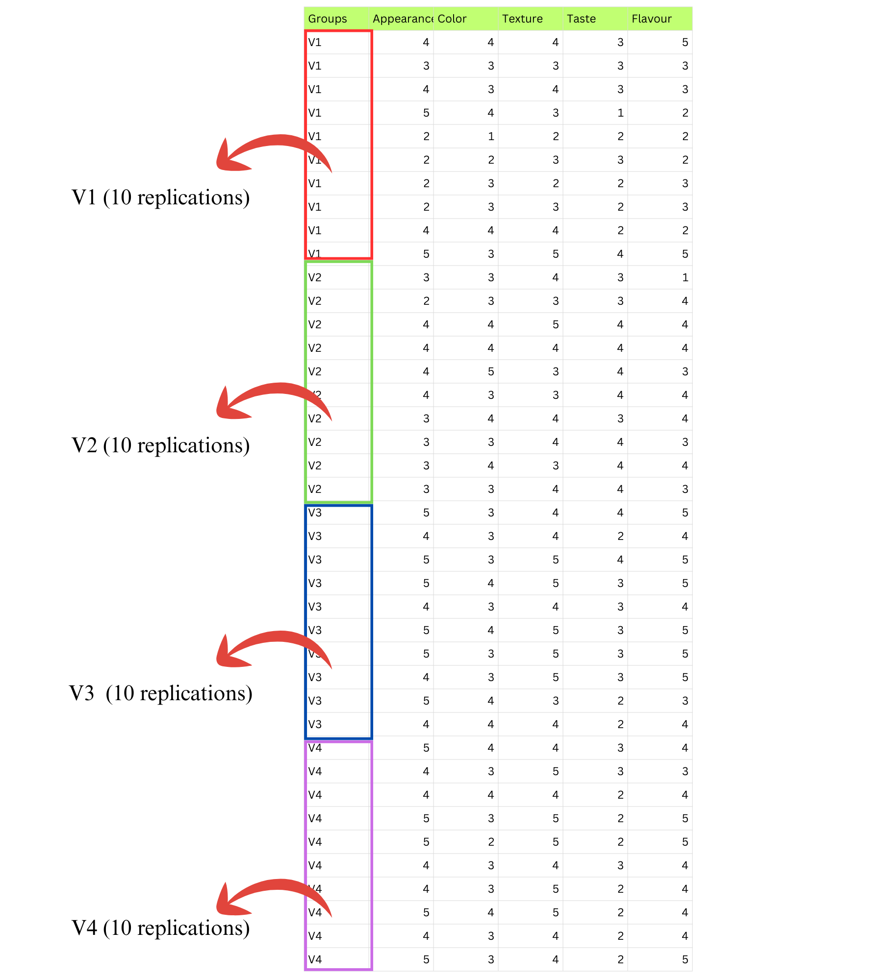
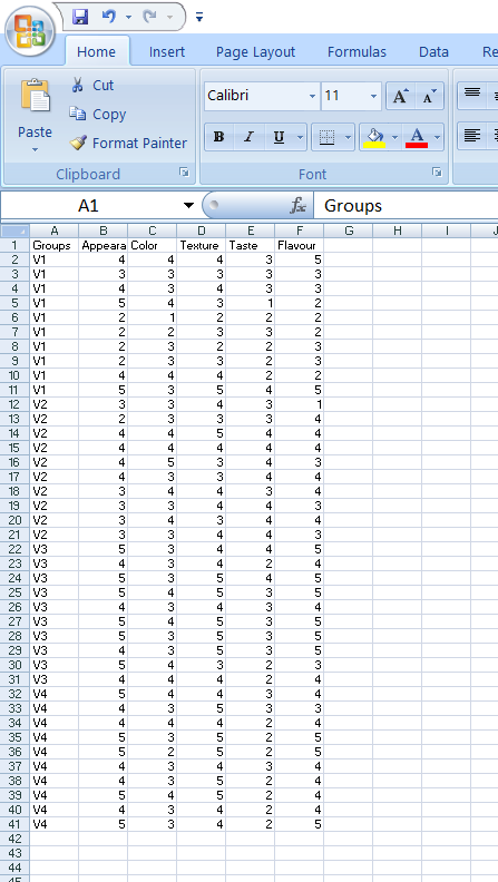
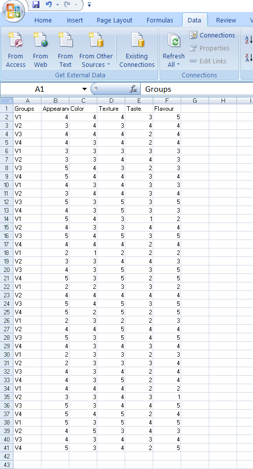
The dataset format required for analysis in RAISINS is illustrated in Figure 2.3.
Preparing data in RAISINS is simple and straightforward. Detailed instructions are provided in Section 3.2. Additionally, model datasets are available within the app for testing purposes, as explained in Section 3.3. See how dataset is arranged for analysis Figure 2.3.
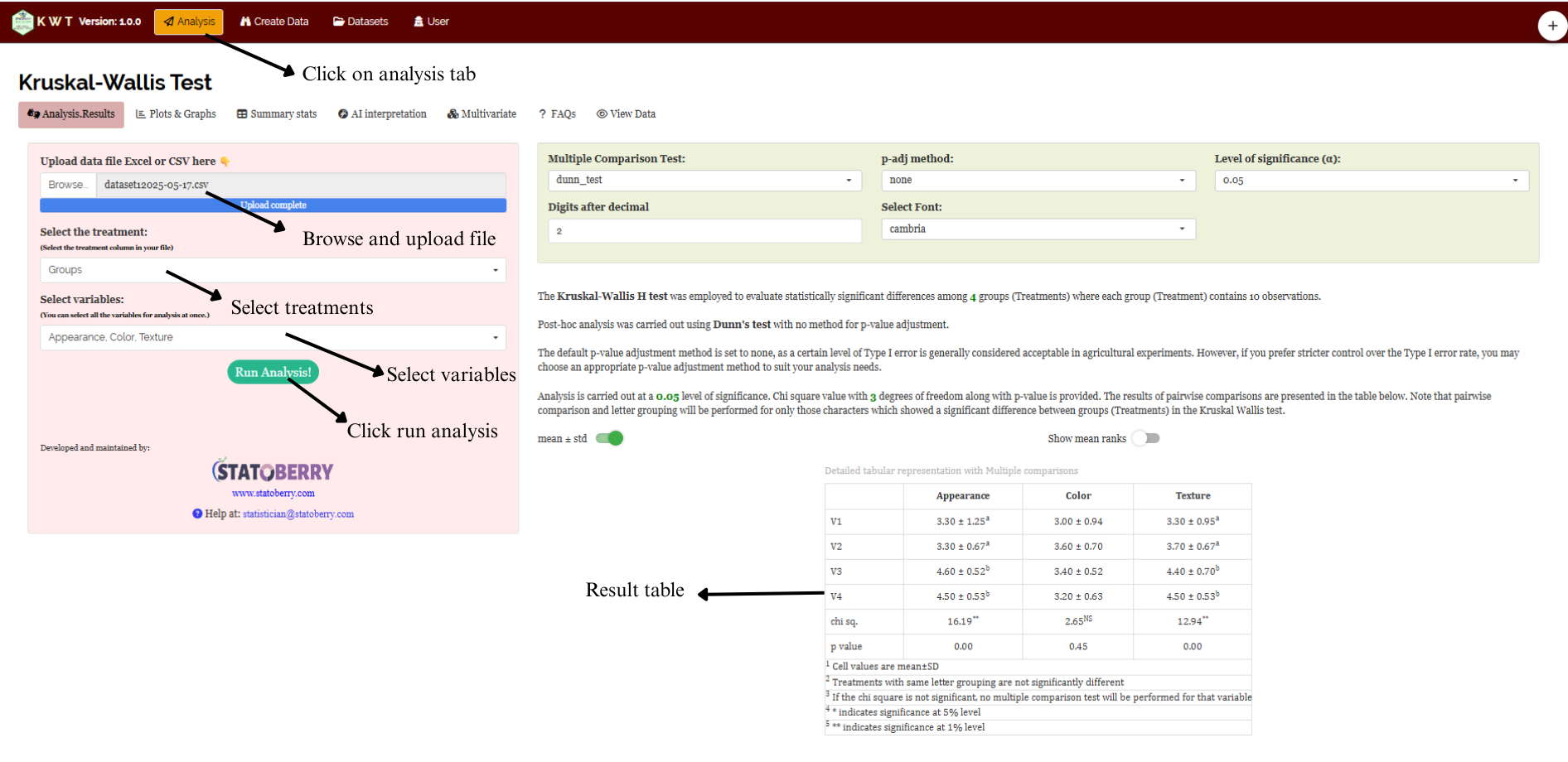
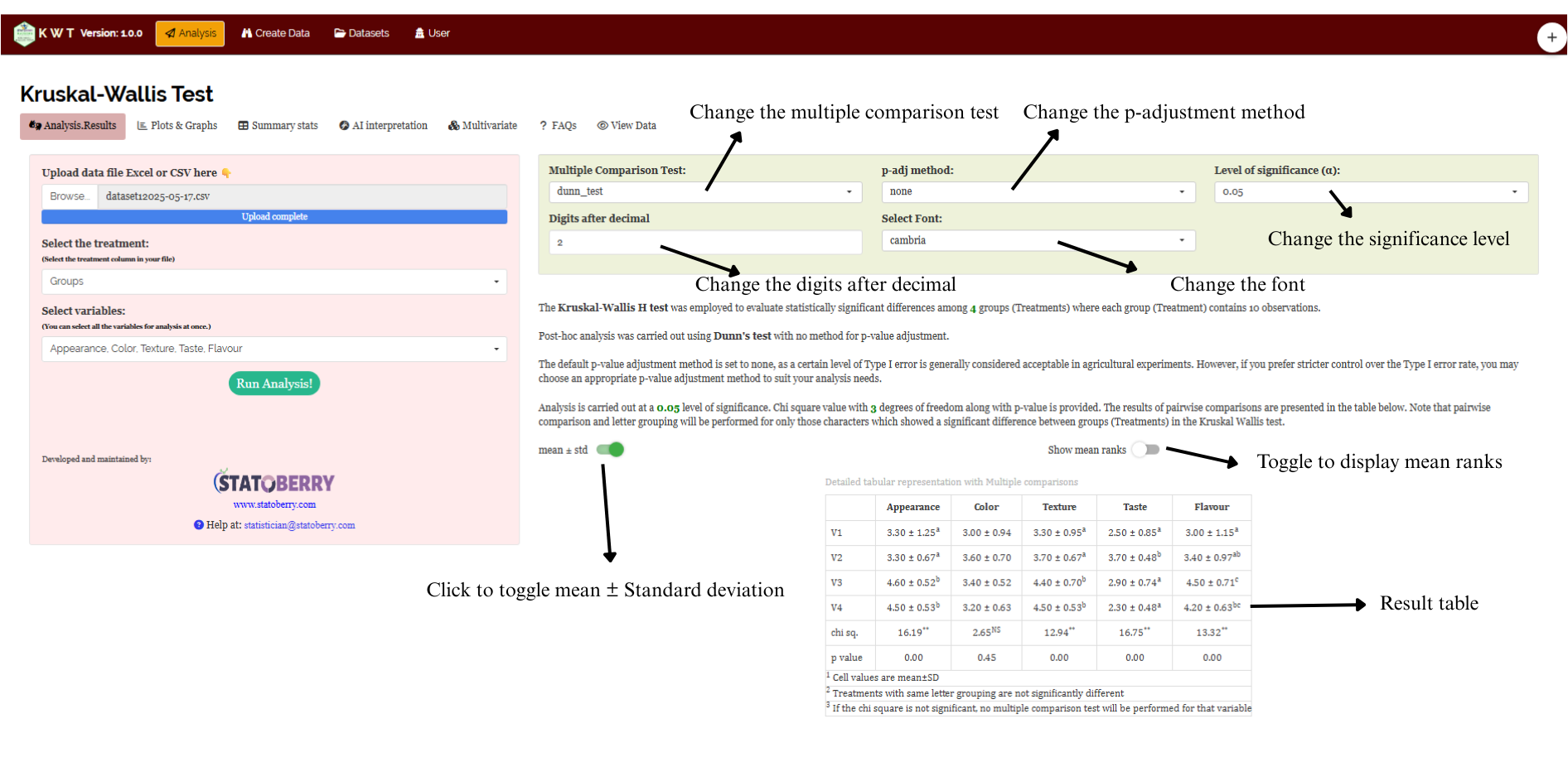
Once the dataset is ready, head onto the Analysis tab in RAISINS and click on Browse and upload the data in csv, xls or xlsx format. After uploading select the treatment and variables of interest(multiple variables can also be selected) and then click on Run Analysis. A complete publication ready results and tables will be generated. Results can be downloaded as pdf, html or word format. See Figure 2.4 for marked Analysis window in RAISINS.
3 Results
RAISINS generates result table in the format given in Figure 3.1 after the analysis.
The result table contains mean ± SD of each observed characters, Chi-square values and p-values showing test significance. The table contains chi-square statistics of each character and it’s significance(p-value). ** indicates significance at 1% level and * indicates significance at 5% level.
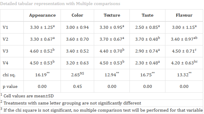
From the result table, it can be concluded that the four drinks differ significantly in terms of appearance, texture, taste, and flavor, as indicated by the significant chi-square values for these characters. However, for the character color, the chi-square value is not significant, suggesting that there is no statistically meaningful difference in color among the four drinks.
Usually while reporting Kruskal Wallis test, mean ranks are also reported so a additional feature to display means ranks is also available in the module.
After a significant result in the Kruskal-Wallis test, a post-hoc comparison is automatically performed to identify which treatment groups differ significantly for each character under study. Dunn’s test will be performed by default, you can change the post-hoc test to LSD (Least significant difference test) by changing from the drop down menu. The results of the post-hoc test are summarized using letter groupings. Treatments that share the same letter are considered on par, meaning their mean ranks are not significantly different.
For example, in the case of the character Color, no letter groupings are shown, indicating that the Kruskal-Wallis test did not find significant differences among the treatments. However, for Appearance, treatments V1 and V2 are assigned the letter ‘a’, while V3 and V4 are assigned the letter ‘b’. This indicates that V1 and V2 form one group with similar appearance, while V3 and V4 form another, significantly different group. Since the mean ranks of V3 and V4 are higher, it suggests that these treatments were rated better in appearance.
You can interpret the results for the other characters in the same way: treatments with the same letter do not differ significantly in their effect on that character, while those with different letters do.
From the results Figure 3.1 , it’s found that appearance wise, drinks V3 and V4 are the best, and by color V2 and V3 are the best. If your objective is to select treatments based on all characters, a multivariate analysis has to be performed. For that click on Multivaraite tab. The results as mentioned in Section 3.1 gives you the best treatment based on all the observed characters.
3.0.1 Customization tabs
In RAISINS, you can easily customize your analysis by adjusting settings such as decimal places, choice of post-hoc tests, p-value adjustment methods, font style, and significance level. These options help tailor the results to your specific needs, as shown in Figure 3.2.
3.0.2 Plots and graphs
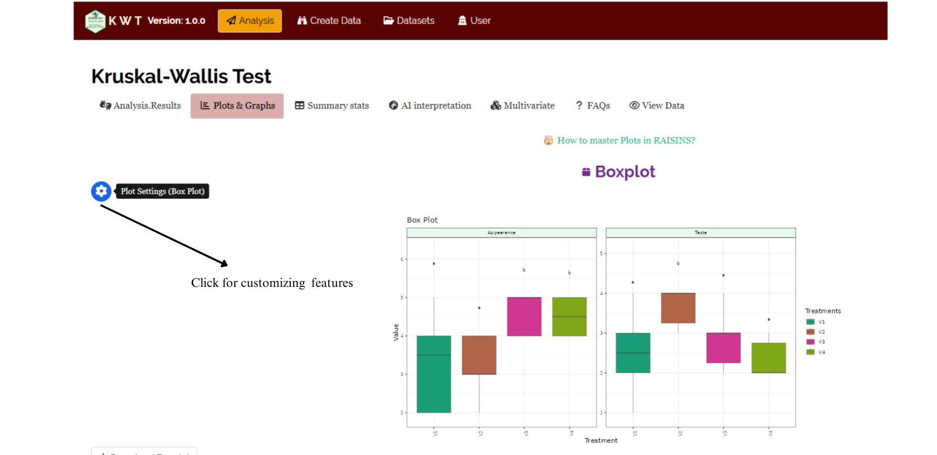
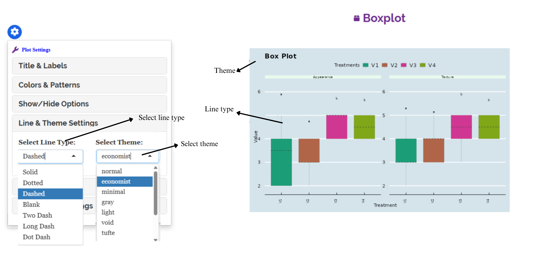
RAISINS is designed for a smooth and hassle-free experience. Once you click the Run Analysis button, all relevant results and outputs appear instantly—leaving no room for confusion. We’ve ensured that every possible plot related to the Kruskal-Wallis test is readily available. Simply click on the Plots & Graphs tab to view them. Each plot comes with a gear icon at the top-left corner, allowing you to customize its appearance. You can also download these plots in high-quality PNG format (300 dpi) for use in reports or presentations.
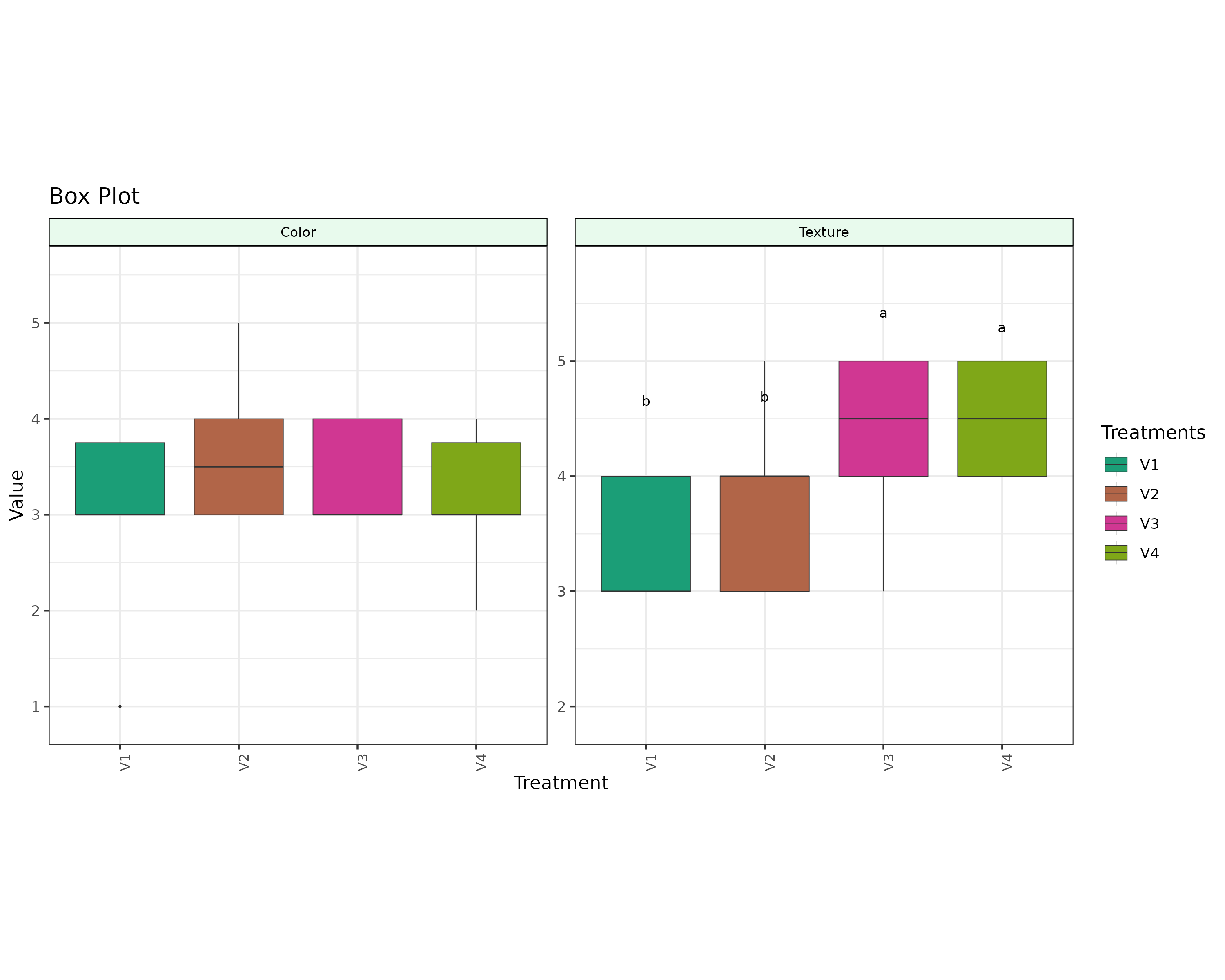
A box plot displays the distribution of data with a five-number summary: minimum, Q1, median, Q3, and maximum. It highlights central tendencies, variability, and outliers with a splash of clarity!
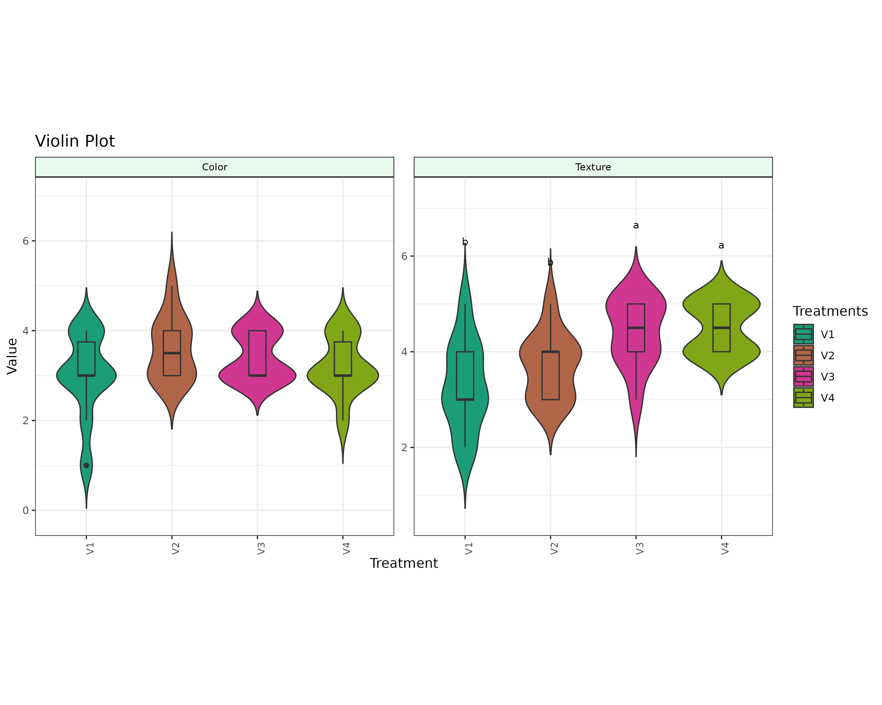
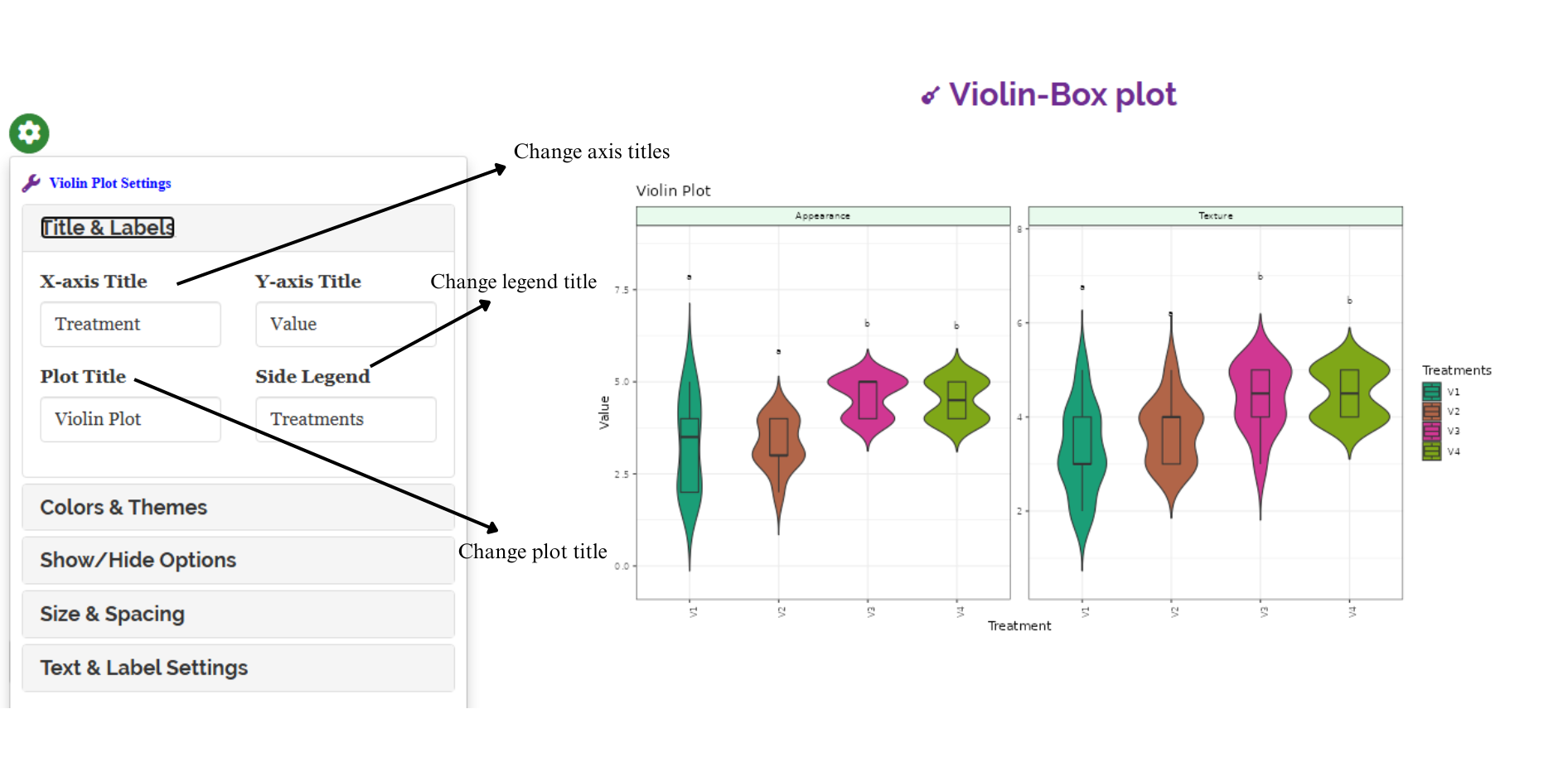
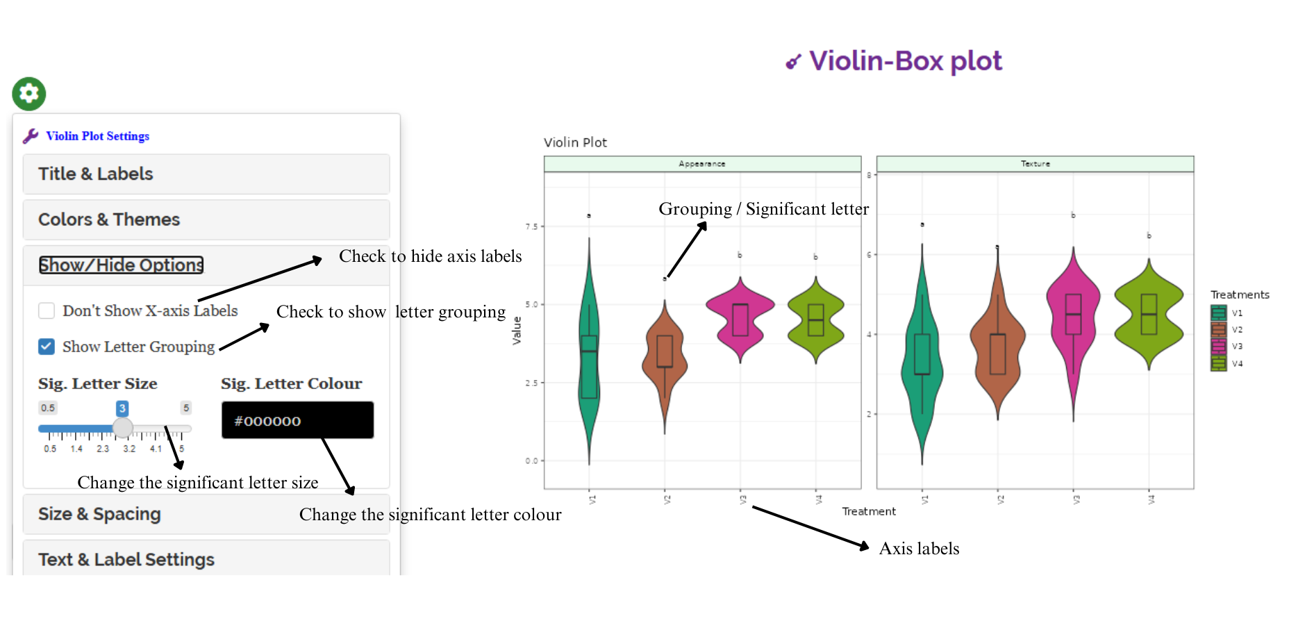
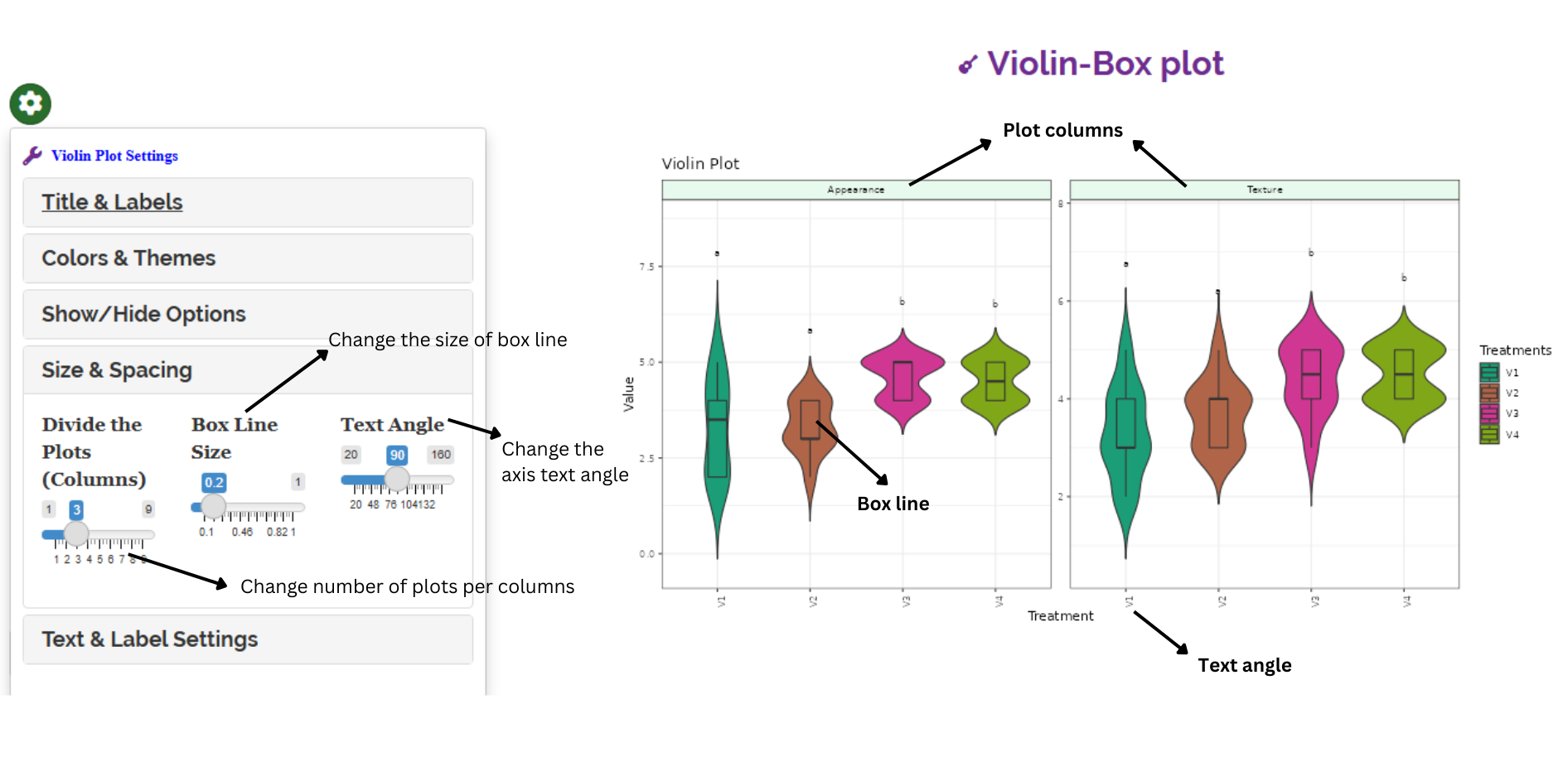
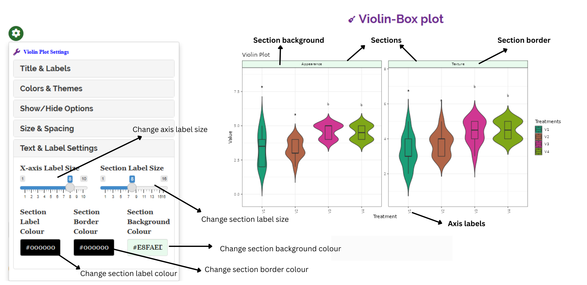
A violin plot combines the box plot and the density trace (or smoothed histogram) into a single display that reveals structure found within the data.
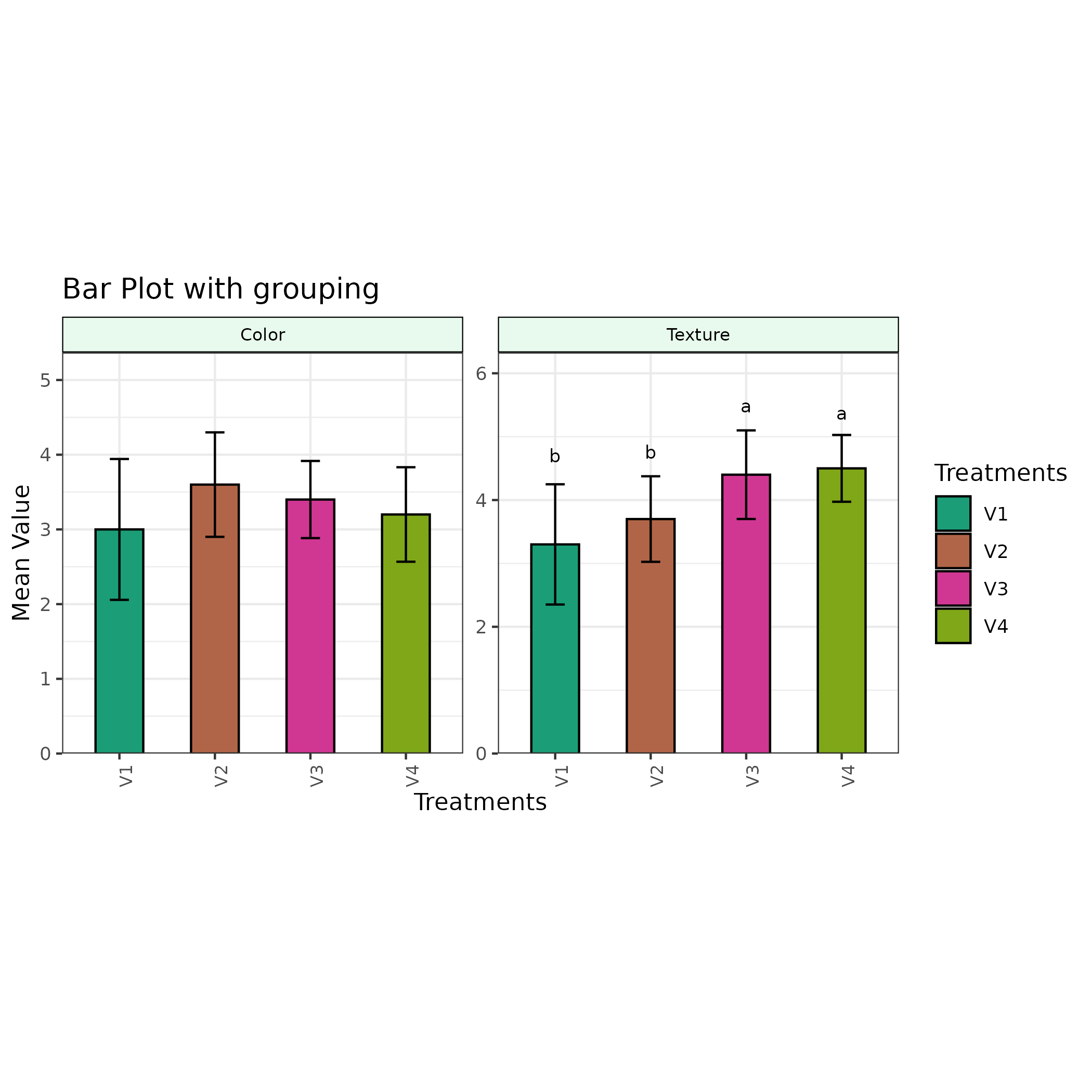
A Bar plot with error bars is a visualization that displays data using rectangular bars, where each bar’s height represents a value (e.g., mean), and error bars indicate the variability or uncertainty (e.g., standard deviation or standard error) around that value. This type of plot is commonly used in scientific and statistical contexts to summarize data and convey reliability..
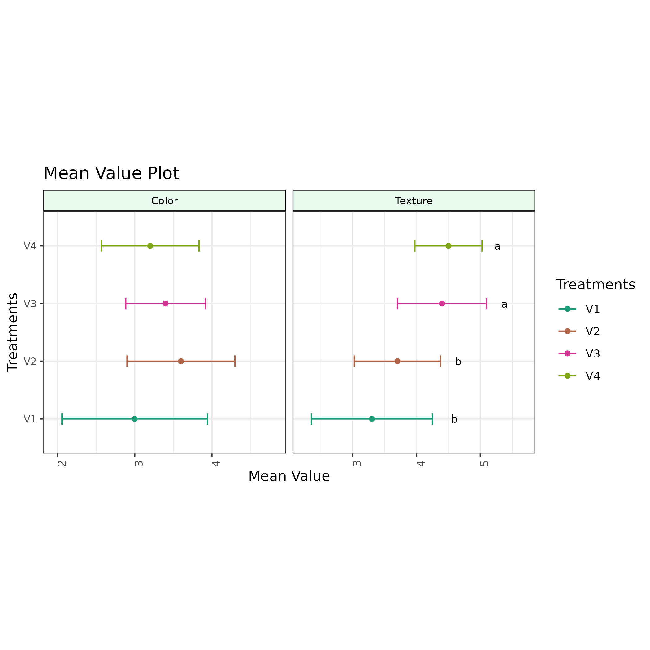
A mean value plot also known as a line plot, is a graphical representation of the average (mean) value of a dataset, often accompanied by error bars that indicates the variability around the mean. It’s used to visualize the central tendency and spread of data.
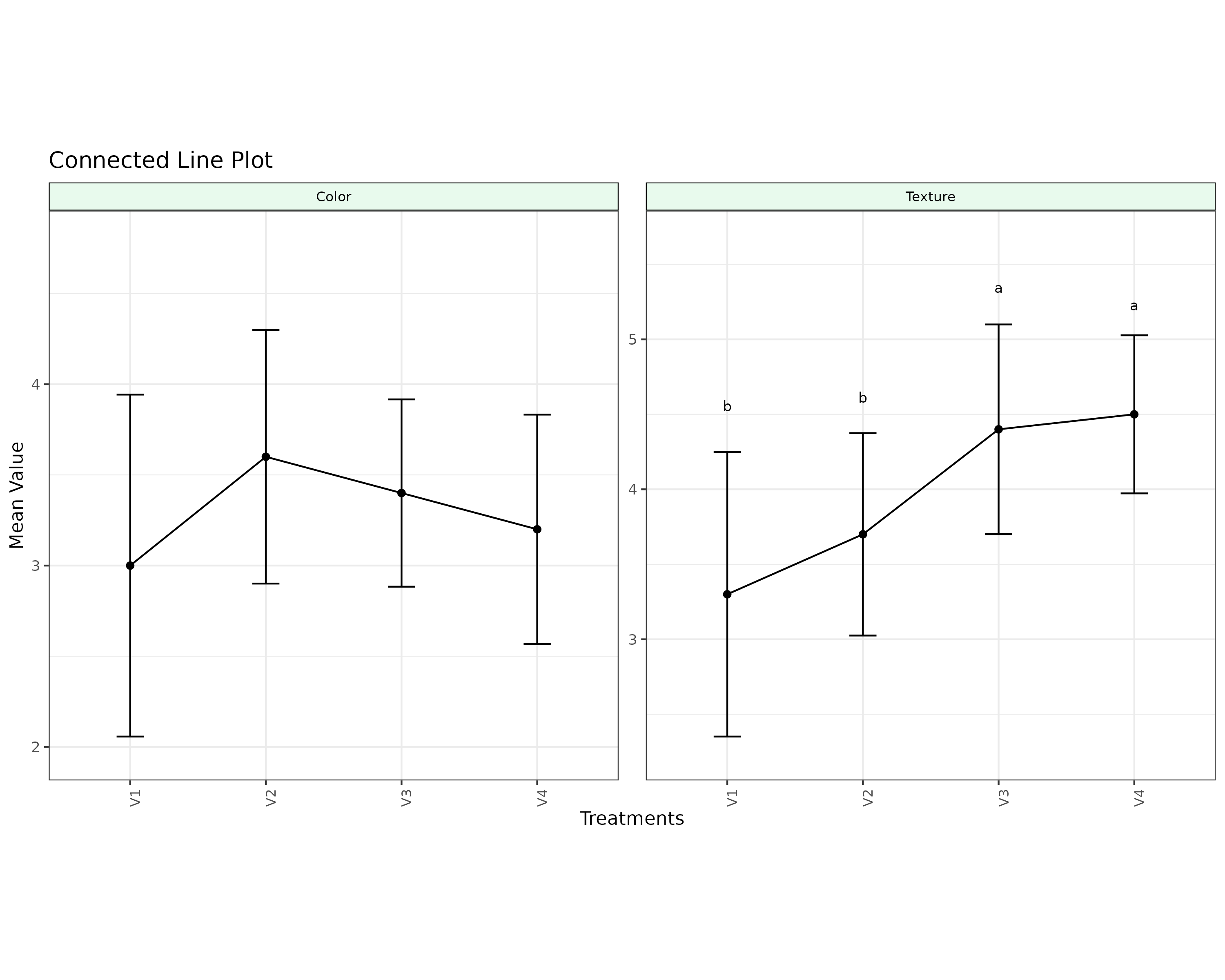
A connected line plot, is a type of chart where mean value points are represented by dots and connected across group by lines, better for comparing between groups, and to see trends and relationships between groups
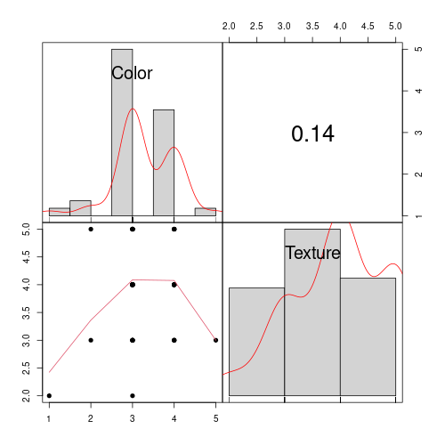
A pairs plot provides three key pieces of information. First, it shows the individual distribution of each variable using a histogram with a smoothed line along the diagonal. Second, it displays the correlation coefficient between each pair of variables, giving a quick sense of their relationship. Third, it includes scatter plots to visually assess how two variables relate to each other. For example, in the example plot, you can see the histogram of the variable Color and Texture, the scatter plot with Color on the x-axis and Texture on the y-axis, and the correlation between Color and Texture, which is 0.14.
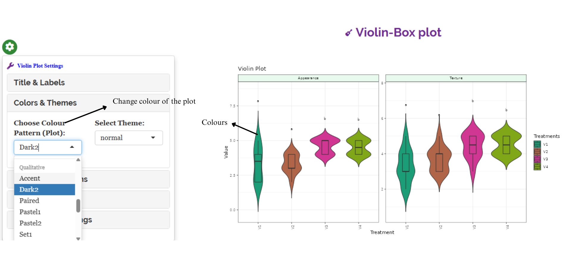
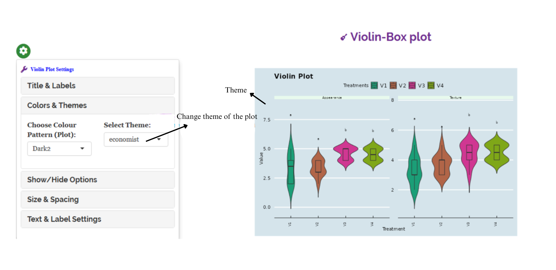
3.0.3 Customizing plots
RAISINS provides user various customization features for the plots to enhance the visualization according to the requirement of the user.Click on the below images to get a clear idea on the customizing features
3.1 Multivariate and AI
The Kruskal-Wallis test is usually used to compare one variable across several groups. Now, In our example of rating four drinks; if we have to identify best drink based on multiple variables (i.e. Appearance, Color, Texture, Taste, Flavour), navigate to Multivariate tab see Figure 3.3. Multivariate analysis in kruskal wallis test helps you to compare different characters simultaneously!. Remember the PCA used for multivariate selection, is an exploratory technique, not an inferential method.
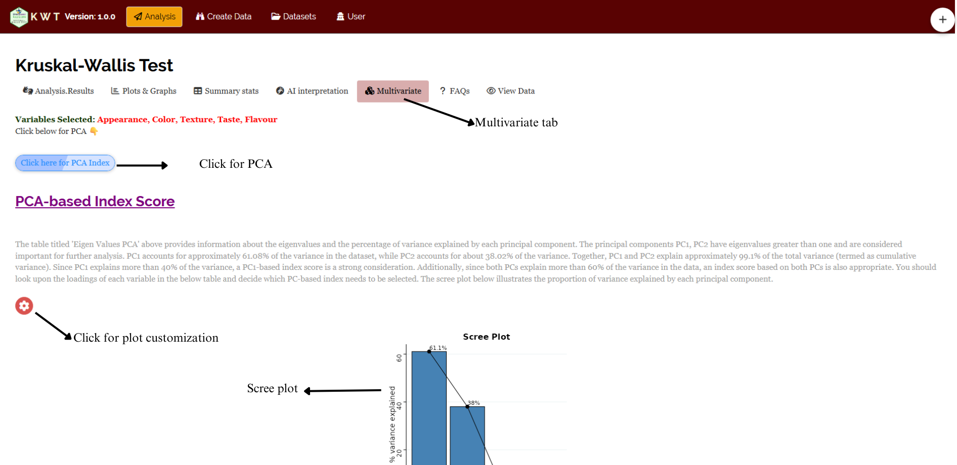
A PCA will be automatically carried out based on the selected variables. PCA results and plots will appear along with automated interpretation.
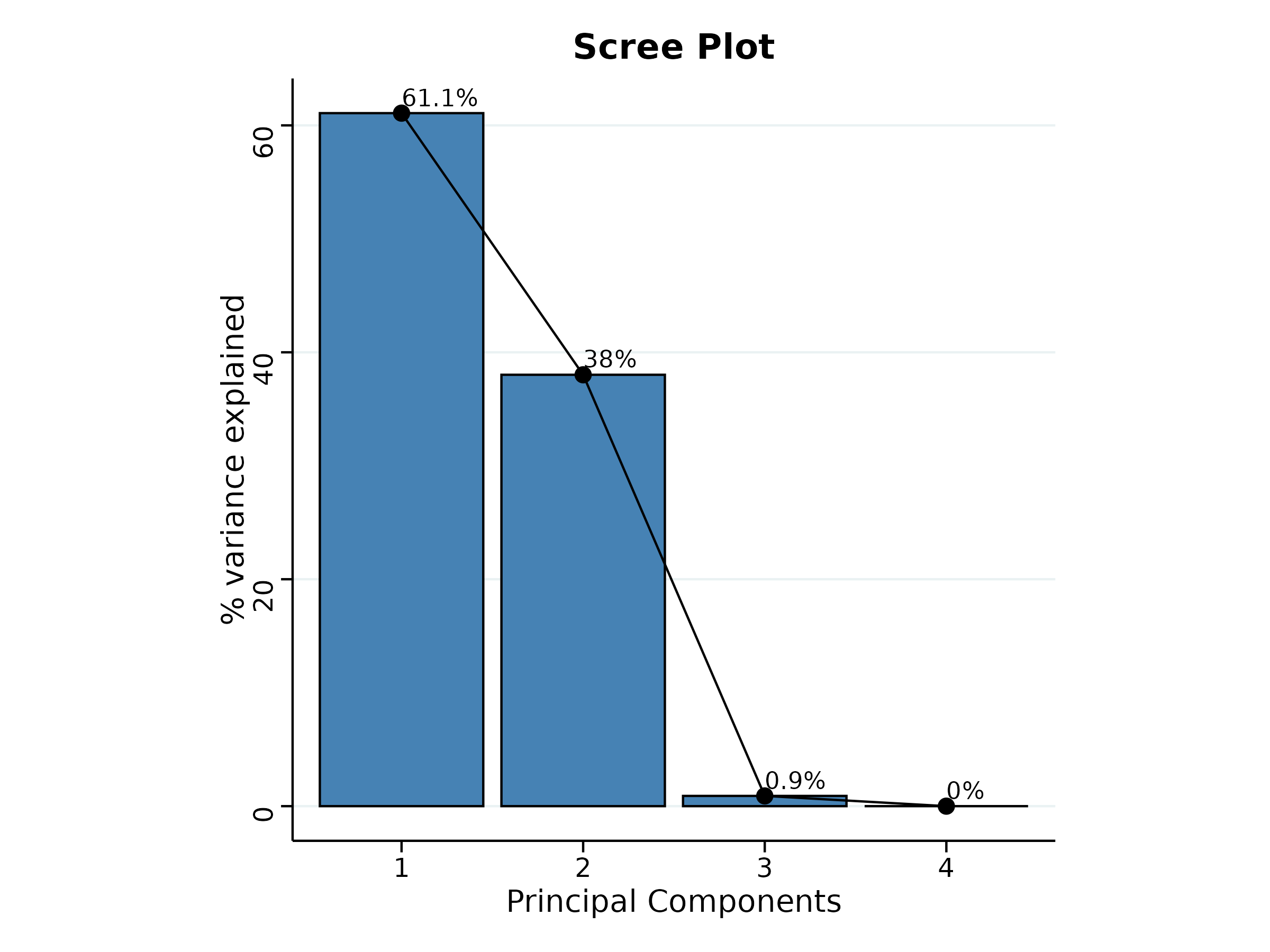
The scree plot given Figure 3.4 illustrates the proportion of variance explained by each principal component. In our example PC1 accounts for approximately 61.08% of the variance in the dataset, while PC2 accounts for about 38.02% of the variance. Together, PC1 and PC2 explain approximately 99.1% of the total variance (termed as cumulative variance). Since PC1 explains more than 60% of the variance, a PC1-based index score is a strong consideration. Additionally, since both PCs explain more than 99% of the variance in the data, an index score based on both PCs is also appropriate. You should also take a look upon the loadings of each variable on the PCs and decide which PC-based index needs to be selected.
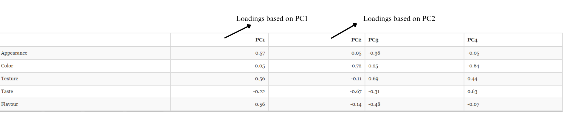
The loadings of each variable on PCs can be seen in Figure 3.5. Here Appearance, Color, Texture and Flavour has positive loading in PC1. So if you want to select best drink based on these four characters, you can use an Index based on PC1. In RAISINS this index is automatically calculated. You can see the index values calculated in Figure 3.6. More mathematical aspects of index construction and scalling can be read in the app itself.
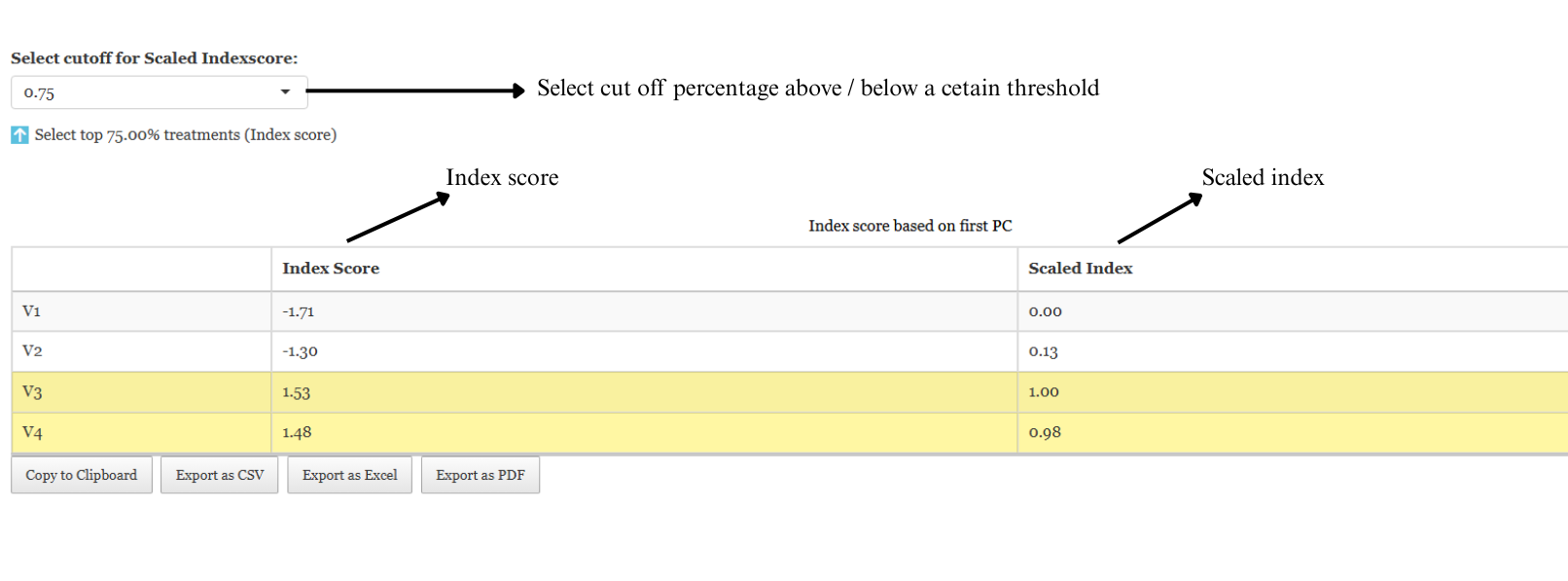
Based on index score it can be seen that, V3 has the highest index followed by V4. So Experimenter can select the drink V3 and V4. Also in some cases when the loadings of prefered variables are negative, a lower index value is preferred. Here to refine your selection, use the ‘Select cutoff for Scaled Index Score’ feature, where you can choose the cutoff percentage to select treatments above or below a certain threshold. The default cutoff is set at 75%. By toggling the up-arrow and down-arrow buttons below the cutoff selection, you can select the top or bottom percentage of treatments as per your preference. Selected treatments are highlighted in yellow in the table below, providing a clear visual cue.
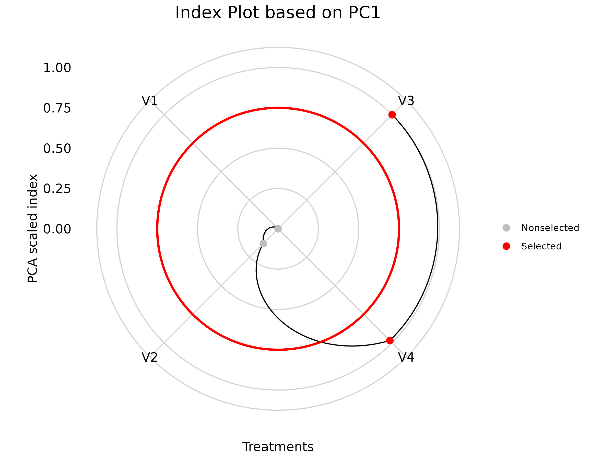
The index plot shown in Figure 3.7, used in the context of Principal Component Analysis (PCA), visually displays the positions of treatments (or groups) based on their index scores—similar to a radar chart. In Figure 3.7, V3 and V4 emerge as the selected drinks based on the four characters under study: appearance, color, texture, and flavour.
Additionally, the biplot in Figure 3.8 clearly shows that V4 and V3 are positioned closer to three key characters—Appearance, Texture, and Flavour—indicating that these treatments scored highly for these attributes. If taste alone is the criterion, V2 emerges as the best candidate, as evident from Figure 3.1. On the other hand, V1 appears to be the least favourable option, having received low scores across all characters.
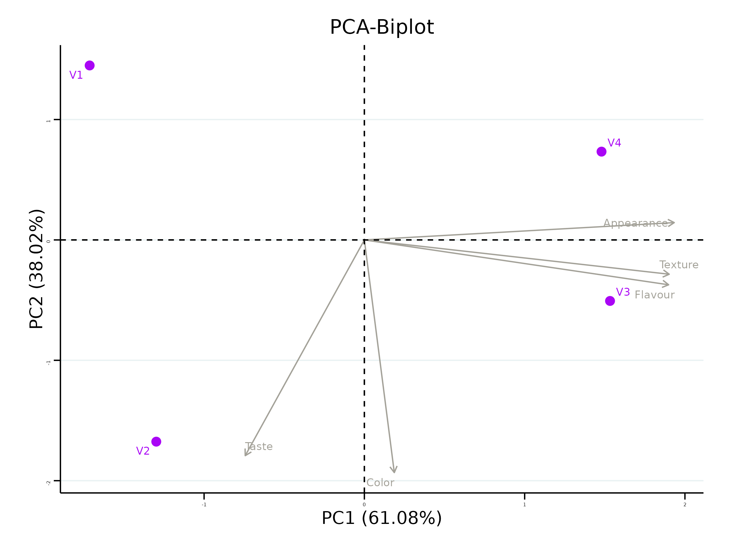
Combining all this information, the experimenter can arrive at an overall conclusion that is statistically sound and contextually relevant to their study.
RAISINS is equipped with an AI-powered RAISINS Assistant designed to assist users in comprehending the outcomes of statistical tests and data analysis. This functionality provides clear and concise summaries of results, identifies statistically significant differences between groups, and offers informed suggestions for potential next steps or interpretations. The AI interpretation given below Figure 3.9
RAISINS enables users to draw meaningful conclusions without requiring advanced expertise in statistics.
3.2 Preparing your data
What truly matters is the quality of your data! As the saying goes, “garbage in, garbage out” — and this holds true for any software. To prepare your dataset for analysis in RAISINS, you have two options:
- Create your dataset in MS Excel
- Build your dataset directly within the RAISINS app
3.2.1 Preparing data in MS Excel
Open a new blank sheet in MS Excel with only one sheet included, and avoid adding any unnecessary content. The dataset should follow a column-based format, where the first column represents the treatment or group to be compared—you can name this column appropriately, such as “Group” or “Treatment.” All characters under study (e.g., Appearance, Texture, Taste) should be arranged in separate columns, and each group should be repeated according to the number of replications. The file can be saved in CSV, XLS, or XLSX format, but CSV is recommended as it is lighter and enables faster loading. Ensure that there are no unwanted spaces in column names or group names. For reference, see the structure shown in Figure 3.10. As illustrated in Figure 2.3, groups must appear repeatedly based on replications, and the data can also be arranged as shown in Figure 3.11.
Dataset Creation Rules
- Column Naming Convention
- No spaces allowed in column names.
- Use underscores (
_) or full stops (.) for separation. - Avoid symbols and special characters like %,# etc
- No spaces allowed in column names.
- Data Arrangement
- Start data arrangement towards the upper-left corner.
- Ensure the row above the data is not blank.
- Start data arrangement towards the upper-left corner.
- Cell Management
- Avoid typing or deleting in cells without data.
- If needed, select affected cells, right-click, and select Clear Contents.
- Avoid typing or deleting in cells without data.
- Column Relevance
- Name all columns meaningfully.
- Exclude unnecessary columns not required for analysis.
- Name all columns meaningfully.
How to Save as CSV in MS Excel
Open Your Workbook
- Ensure your data is arranged properly with only one sheet.
Click ‘File’ Menu
- Go to the top-left corner and click on File.
Choose ‘Save As’ or ‘Save a Copy’
- Select the location where you want to save your file.
Set File Type to CSV
- In the ‘Save as type’ dropdown menu, choose CSV (Comma delimited) (*.csv).
Name Your File
- Enter a relevant file name without spaces (use underscores if needed).
Click ‘Save’
- Click Save to export the file.
💡 Tip: Before saving, double-check that your data is on the first sheet and follows the required format (e.g., no empty rows above the data, meaningful column names).
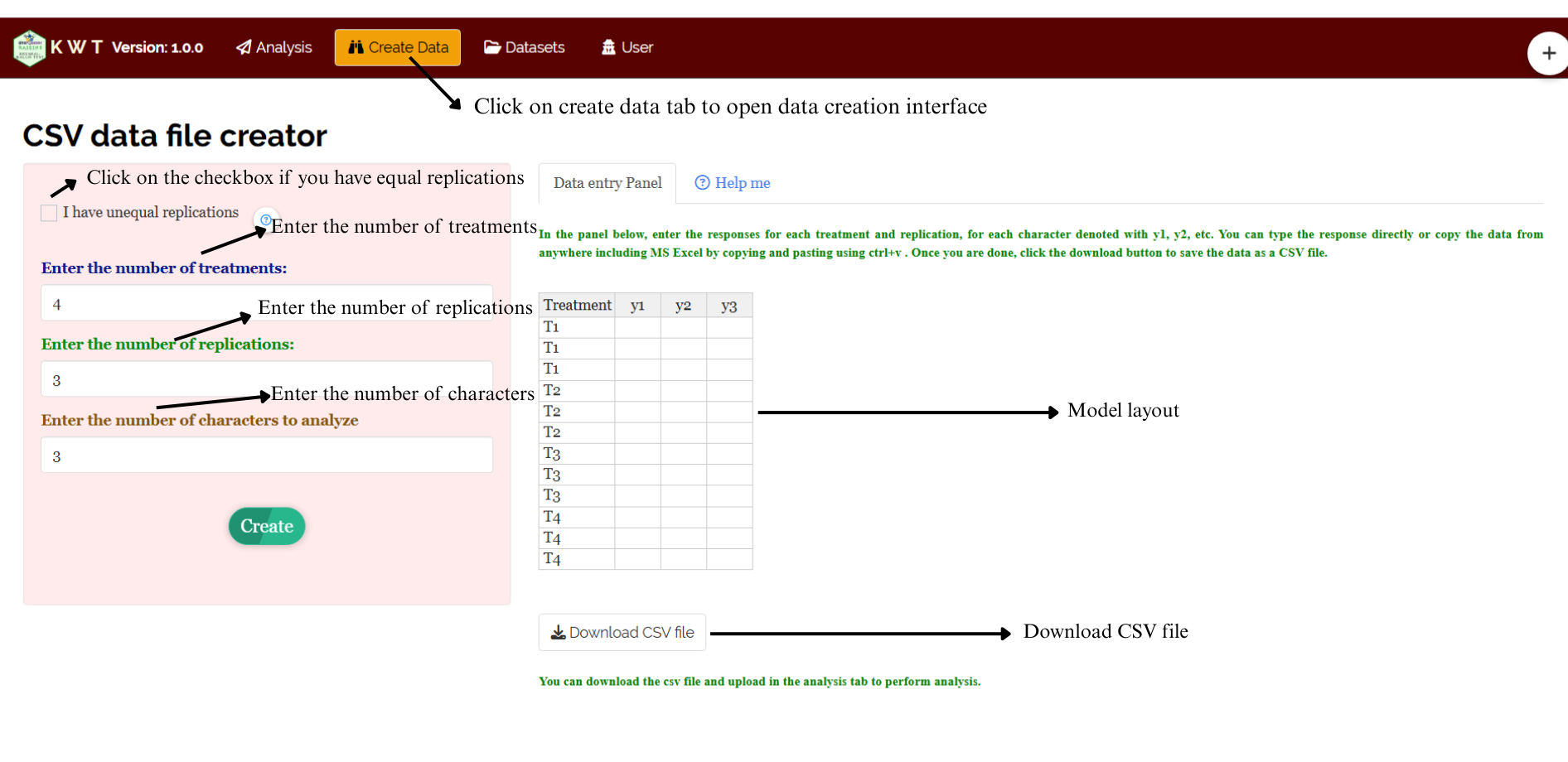
3.2.2 Creating dataset in RAISINS
If you’re unsure about the correct format for creating a dataset, don’t worry—Raisins offers an option to create data directly within the app using the prescribed template. Here’s how:
➡️Navigate to the Create Data Tab
➡️ Select the number of Treatments
➡️ Select number of Replications
➡️Click onCreate button**
Model layout will appear as shown in Figure 3.12. Now you may enter the observations manually into the CSV file once downloaded, or paste the observations straight into the file provided. Once you have entered the observations in the layout, download the csv file and upload in Analysis tab!
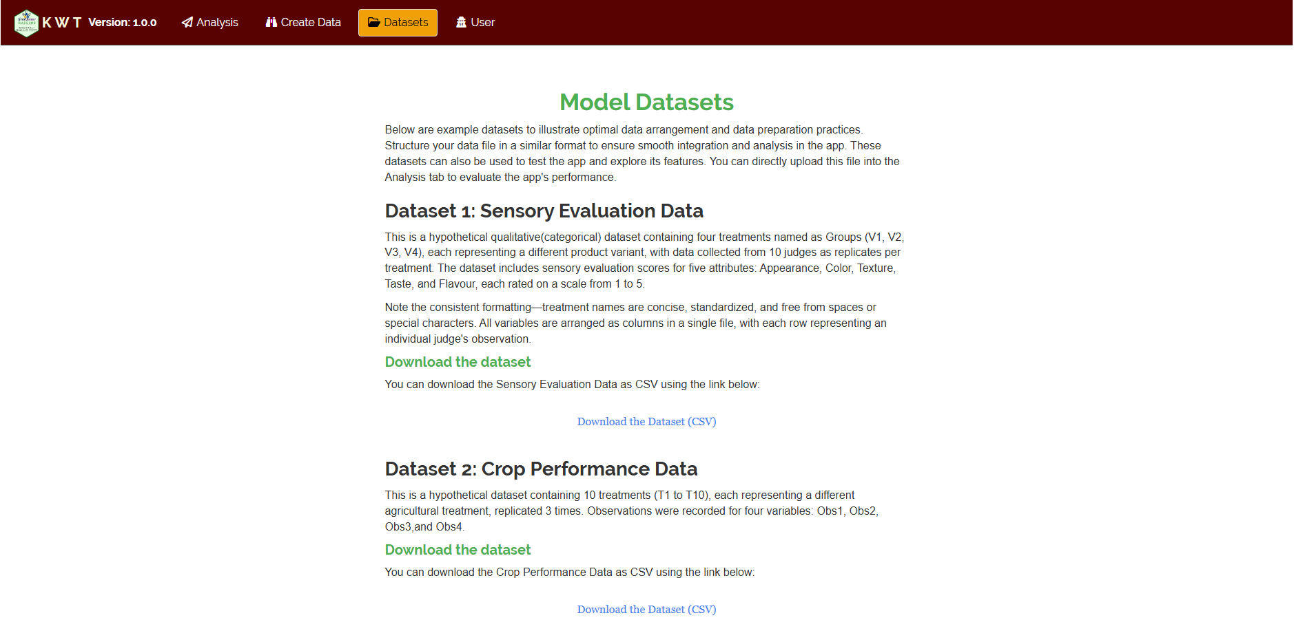
3.3 Model Datasets
To test the app or better understand the data arrangement, we provide model datasets within the app. You can download them from the Datasets tab.
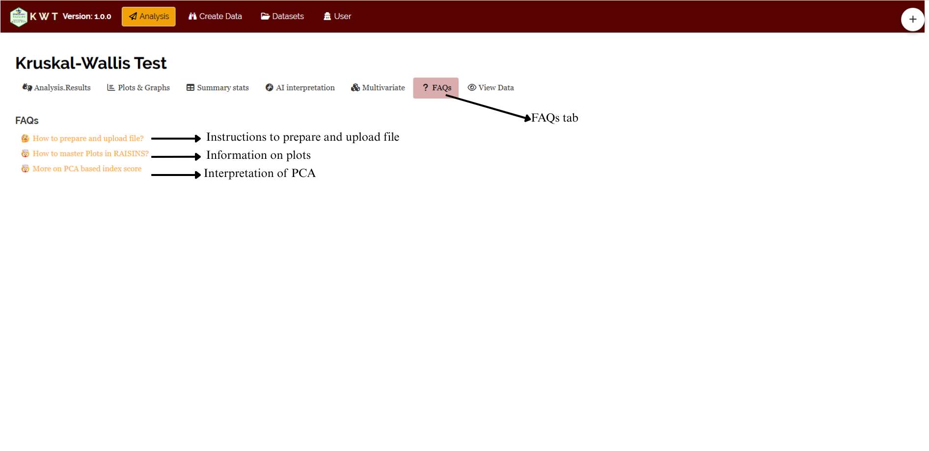
3.4 FAQ’s
The app includes a dedicated FAQ tab to help clarify common doubts and guide users through various features. This section provides detailed answers to frequently asked questions, offering additional information and helpful tips to ensure a smooth user experience. If you’re ever unsure about how something works, the FAQ tab is a great place to start.
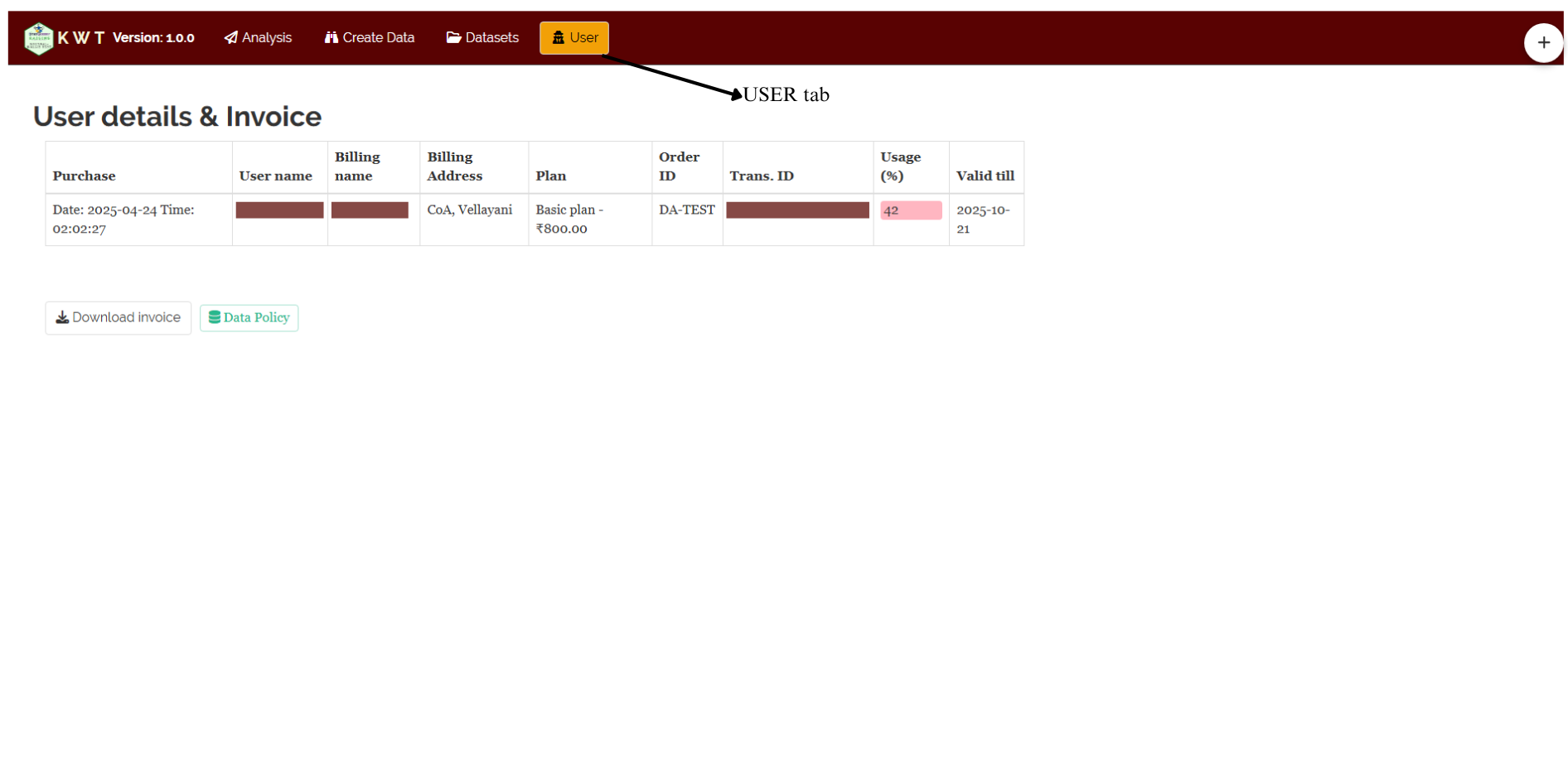
3.5 User
You can find all your account details—including usage percentage, plan validity, subscription type, and billing information-under the User tab. This section also allows you to download your GST invoice. We adhere to a strict data policy: each time you log in, a temporary instance of the app is created exclusively for you, which is automatically terminated when you log out. No uploaded data or generated results are stored, ensuring complete privacy and data security.